The Game of Life With Macroeconomic Stimulus

Agent-Based Models

The origins and early years

According to Wikipedia an agent-based model (ABM) is

ABM: class of computational models for simulating the actions and interactions of autonomous agents (both individual or collective entities such as organizations or groups) with a view to assessing their effects on the system as a whole.

A cellular automaton is a particular class of ABM. It is a discrete dynamical model used and studied in a variety of fields: computer science, mathematics, physics, complexity science, theoretical biology among others. Compared to ABM’s, Cellular Automata are more structured: ABM agents are heterogeneous and can interact in complex ways. A cellular automaton consists typically of a regular grid of cells, each one in one of a finite number of states.

Both of these concepts originate in the 1940s in the work of Stanislaw Ulam and John von Neumann while they were working at Los Alamos National Laboratory studying nuclear fission. Underlying the viability of this type of model is the development of techniques to use random numbers in computation: Namely the Monte Carlo method.

In a recent post and Open Risk Academy course we discussed the important role of simulation in modelling credit contagion in economic networks. In this post we take a step back and look at a broader class of systems such ABM and Cellular Automata

Adoption in Economics and Finance

ABM techniques find a number of applications in economics but are very far from mainstream. A recent review of the most notable work in a variety of economic contexts was given by ¹ (which we summarize here):

• The earliest application seems to be the 1957 work by Guy Orcutt who proposed a new model which consists of various sorts of interacting units which receive inputs and generate outputs ². This work is now credited to have given birth to the field of Microsimulation.
• Another famous application of ABM’s is Thomas Schelling’s work on racial segregation ³. He demonstrated how, in a simple cellular structure with agents following simple rules of thumb, a pattern of segregation might naturally emerge. The model’s predictions closely matched locational patterns in real cities and communities.
• In the 1980s, Robert Axelrod applied ABMs to game theory ⁴ investigating, for example, the optimal behavioural response of agents in repeated games
• Post the Great Financial Crisis ABMs have been used to explain irregularities in financial markets, such as crashes and fat-tailed asset prices distributions ⁵.

A further list of papers proposing heterogeneous models is available here

Modern ABM Frameworks

There are various current efforts to create flexible and general purpose frameworks for modelling Agent Based systems. The following list is indicative (with links to an open source repository where available):

• Complexity Research Initiative for Systemic Instabilities (CRISIS), an open source collaboration between academics, firms, and policymakers (Klimek (2015)).
• EURACE, a large micro-founded macroeconomic model with regional heterogeneity (Dawid (2012)).
• MESA, an agent-based modeling framework in Python 3+
• abcEconomics, an Agent-Based Computational Economy platform that makes modeling easier
• Agents.jl, an agent-based modeling framework in Julia
• pandora, a C++/Python Agent-Based Modelling framework for large-scale distributed simulations

The Game of Life - with a twist

The Game of Life, also known simply as Life, is a cellular automaton devised by the British mathematician John Horton Conway in 1970. It has been extremely successful in popularizing the concept of cellular automata and is even today a very common programming task for first time developers.

The Standard Setup

Entities are arranged on a regular grid (that can be thought of extending to infinity or wrapping up in periodic fashion). Each entities is either alive or dead (two states). Evolution takes place in global updates of all states according to prescribed rules based on the live of dead status of neighboring cells.

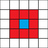
The neighborhood

The evolution of the life and death of a given cell in Conway’s original version derives from the state of the neighboring cells, in particular those forming the so-called Moore neighborhood:

The rules

The standard rules are as follows:

• Any live cell with fewer than two live neighbours dies, as if by under-population
• Any live cell with two or three live neighbours lives on to the next generation
• Any live cell with more than three live neighbours dies, as if by overpopulation
• Any dead cell with exactly three live neighbours becomes a live cell, as if by reproduction

Conway chose his rules carefully, after considerable experimentation, to meet these criteria⁶:

• There should be no explosive growth
• There should exist small initial patterns with chaotic, unpredictable outcomes.
• There should be potential for von Neumann universal constructors.
• The rules should be as simple as possible, whilst adhering to the above constraints

In order to implement the rules flexibly we split them as follows:

    // Birth zones by right-crowding
    // Outside zone, remain dead
    if (R(i, k - 1) == 0 and (live > Death2LifeUpper or live < Death2LifeLower)) {
        R(i, k) = 0;
    }
        // Inside zone, rebirth
    else if (R(i, k - 1) == 0 and not(live > Death2LifeUpper or live < Death2LifeLower)) {
        R(i, k) = 1;
    }
        // Death zones by over or under-crowding, die
    else if (R(i, k - 1) == 1 and (live > Life2DeathUpper or live < Life2DeathLower)) {
        R(i, k) = 0;
    }
        // Right-crowding, stay alive
    else if (R(i, k - 1) == 1 and not(live > Life2DeathUpper or live < Life2DeathLower)) {
        R(i, k) = 1;
    } else {
        cout << "ERROR" << std::endl;
    }

Parameterizing the rules

In the above snippet we introduced parametric thresholds:

    // Initial Rules
    int Life2DeathUpper = 3;
    int Life2DeathLower = 2;
    int Death2LifeLower = 3;
    int Death2LifeUpper = 3;

Now we can recast the rules as follows:

For a “live” count in the Moore neighborhood,

• A live cell dies if the count exceeds Life2DeathUpper
• A live cell dies if the count falls below Life2DeathLower

On the other hand, a dead cell revives only if the count exceeds Death2LifeLower but is lower than Death2LifeUpper

The Typical Evolution

The Game of Life is not stochastic. Once we specify the initial state, the evolution is deterministic and unique.

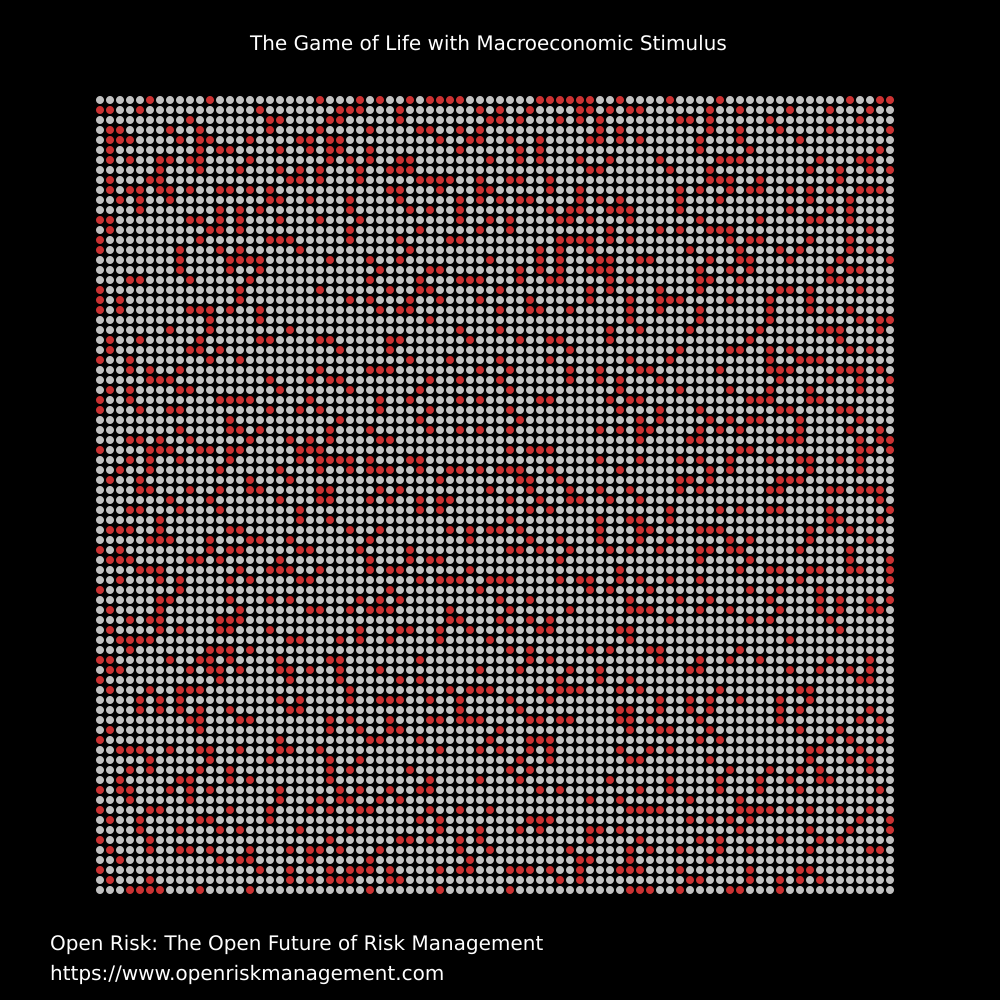
The above image shows an initial randomly seeded configuration.

It is not easy to define “typical evolution” as it depends on the initial configuration of live cells. If by “typical” we mean the development following a random distribution of initially live states then it proceeds qualitatively as follows:

• a period of cleansing during which the initially unviable configurations quickly die out
• a period of localized growth during which some configurations may flurish and grow
• a period of decay which may lead to a static residual configuration (with possible periodic elements)

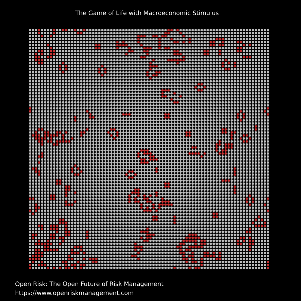
The above image shows a typical, slowly dying configuration

Gosper’s Glider Gun

An example of complex periodic elements that might emerge during the evolution of the CA is Gosper’s glider gun.

“Macroeconomic” Stimulus

While repeated experiments (or maybe brilliant reasoning!) may reveal interesting emergent behavior, the typical outcome is rather bland. How can we intervene to maintain a level of activity?

Modifying the rules

The idea is to modify the rules by widening the window of scenarios where a dead cell revives. Instead of exactly three, we include 2, 3 and 4.

    if (LiveCount < Threshold1) {
        Death2LifeLower = 2;
        Death2LifeUpper = 4;
    }
    if (LiveCount > Threshold2) {
        Death2LifeLower = 3;
        Death2LifeUpper = 3;
    }

Our “intervention” into the CA algorithm violates the local nature of the system. It resembles policy based on macro-economic considerations (aggregate observables) that take the global picture of the system into account. But the rule change is indeed local, in that sense that the new live cells are produced organically and are not seeded from outside as “helicopter money”.

Boom and Bust

The video shows the impact of the adjusted rules. Every time activity drops below a predetermined threshold, the rules are relaxed to allow more cell regeneration. During that period growth is actually explosive! Once another predetermined level is reached (which happens over a few periods), the rules revert to the normal.

The result of the “intervention” is that the evolution continuously bounces between the two stimulus thresholds. Notably, there is very little room for emergent behavior.

References

-
The dappled world, A.Haldane (Bank of England Speech), 2016 ↩︎
A new type of socio-economic system, G.Orcutt, 1957 (Available @ International Journal of Microsimulation, ↩︎
Dynamic models of segregation, T.Schelling, Journal of mathematical sociology, 1971 ↩︎
The complexity of cooperation: Agent-based models of competition and collaboration, R.Axelrod, Princeton University Press, 1997 ↩︎
Getting at systemic risk via an agent-based model of the housing market, J Geanakoplos, et al, The American Economic Review, 2012 ↩︎
Wikipedia reference to private Conway community to mailing list ↩︎
Comment
If you want to comment on this post you can do so on Reddit or alternatively at the Open Risk Commons. Please note that you will need a Reddit or Open Risk Commons account respectively to be able to comment!