Input-Output Models as Graph Networks
We discuss the relation of economic input-output models with graph theory and networks
Course Objective
The objective of the course is to discuss the relation of economic input-output models with graph theory and networks.
The course is now live at the Academy.
Pre-requisites
Basic knowledge of input-output models and graph theory would help to get the most out of the course but is not strictly required.
Summary of the Course
What we cover in this course:
- Step 1. In this step we discuss in more detail the motivation for the course and provide a very brief introduction to the graph theory to establish the notation.
- Step 2. In this step we explore the duality between graphs and matrix representations.
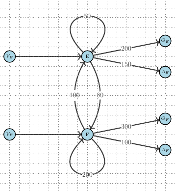
- Step 3. This step introduces the concept of Qualitative Input-Output Analysis
- Step 4. In the fourth step off the course we discuss Sources, Sinks and Conservation Laws
- Step 5.In the final step of the course discuss and interpret in graph terms the typical question one wants to answer with an IO model: what happens if there is new set of final demands?
Get Started with the Course
The course is available at the Academy.