Monte Carlo Simulation of the US Electoral College

The role of simulation in risk management and decision support

A Simulation is a simplified imitation of a process or system that represents with some fidelity its operation over time. In the context of risk management and decision support simulation can be a very powerful tool as it allows us to assess potential outcomes in a systematic way and explore what-if questions in ways that might otherwise be not feasible. Simulation is used when the underlying model is too complex to yield explicit analytic models (An analytic model is one can be “solved” exactly or with standard numerical methods, for example resulting in a formula).

Complexity in a system arises from many distinct architectural aspects:

• the large number of elements in the system (e.g. the number of atoms in a cup of tea)
• the many internal states per element (e.g. all possible configurations of chemicals inside a living cell)
• the many interactions between elements (e.g. all possible transactions of a company in different markets)

In fact as the number of elements in a system grows, even very simple considerations become intractable because of the large number of possible combinations in which things can play out. The phenomenon is sometimes called the combinatorial explosion. A particular type of simulation that comes handy when trying to handle combinatorial complexity is the so-called Monte Carlo Simulation. It is a concrete (and in its essence quite simple) mathematical technique whereby multiple scenarios are constructed and analysed via the generation of artificially generated (via a digital computer) using random numbers. These random numbers try to capture the evolution possibilities available to each element of the system in separate future scenarios. Iterating over the entire system and over repeated scenarios gives us insights into what is the distribution of various outcomes of interest.

In this post, we illustrate the principle in a simple setting where will use Monte Carlo to explore the rules and mechanics of the US Electoral College system. Specifically we will simulate possible outcomes in what is a very simplified and politically agnostic setting.

Spoiler alert, there is nothing to be learned about politics here!

The rules of the US Electoral College System and the “paths to victory”

The United States Electoral College is the group of presidential electors required by the US Constitution to form every four years for the sole purpose of electing the president and vice president. Each state appoints electors according to its legislature. Of the current (2020) 538 electors, an absolute majority of 270 or more electoral votes is required to elect the president and vice president. The distribution of electoral votes per state is shown in the following map (This a Hexagonal cartogram of the number of United States electoral college votes for each state and District of Columbia since 2012 by CMG Lee based on a National Geographic original)

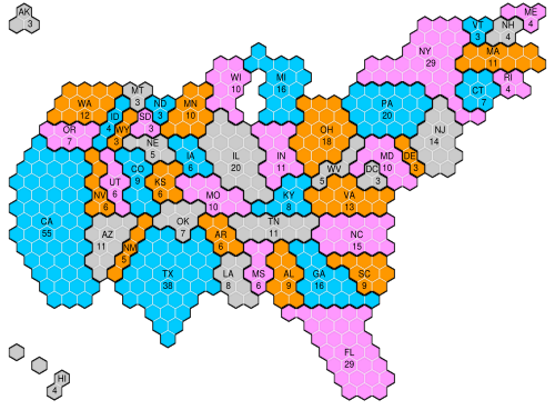
We notice some important features of the electoral vote distribution. It varies a lot per state, ranging from a minimum of 3 to the largest number (55). We see that the so-called “paths-to-victory”, namely the precise combination of states that leads to a winning result is, a-priori, without making any assumptions, quite difficult to estimate. There is namely a vast number of possible combinations of states that leads to the required 270 majority. This is precisely the combinatorial challenge for which Monte Carlo is very suitable. Lets see how we can setup a rudimentary simulation framework.

Constructing a simulation framework

We setup a simulation framework as follows:

• For each election round we go over all states $i$ and we flip a coin. If the coin comes head, the state vote count $v_i$ is allocated to one party. If it comes tails, it gets allocated to the other party (Which one it is which does not matter for our discussion here! The analysis is complete symmetric)
• Each simulation round represents one election.
• We calculate 1000 scenarios (arbitrary choice: we can keep simulating until we exhaust our computing budget). With four years per real election period we span one millennium worth of elections! This fact illustrates a point that can be sometimes confusing about simulations. The successive samples are not a sequence of future elections, but rather alternative possible realization at a current timepoint. The two viewpoints might overlap (hence the confusion) if we assume that the system does not change at all over time.
• We sum the electoral votes per scenario and compare whether the party we monitor has “a path to victory” them against the 270 threshold. Expressed in terms of random variables, we have state random variables $V_i$ and a total electoral vote achieved by one party $V_T$.

Expressed mathematically as:

$V_T = \sum_{i=1}^{51} V_i$

The complications we ignore

There are many complications of the actual US electoral college mechanics that do not concern us here, as our purpose is not to create a political simulation but rather illustrate Monte Carlo in a somewhat realistic setting. Maybe it is worth enumerating some such complications, to illustrate the type of challenges more realistic analyses would have to grapple with:

• The number of parties competing in elections is not confined to just two
• Two states do not follow the winner-takes-all rule for electoral votes and may split the votes
• The unbiased (50%/50%) chance of a political party to secure the majority of votes is very far from truth, although determining this more precisely is very far from trivial!
• The assumption of independent draws in different states is obviously also very far from the truth. In general, we would expect strong correlation between outcomes, though again the actual dependency might be very difficult to establish.

Setting up the Stage

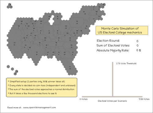
The next diagram illustrates the canvas on which we will project the simulation results. For each simulation (Election Round), the states will be colored with the corresponding winning party. The total votes gathered will be summed up and shown under Sum of Electoral Votes. The Absolute Majority Rate keeps track of the success rate of exceeding the 270 threshold. This is simply the ratio of the number of scenarios exceeding the threshold up to this point of the simulation, versus the current simulation count.

Below these aggregate numbers we will see the histogram of realizations as it gets populated with scenarios. Each simulation gets represented by a small rectangle. It is placed on the x-axis depending on the number of total votes (0 to 538). If the same cumulative vote count has been observed before, the rectangle location is bumped upwards in the y-axis. Hence a vote count that appears many times will create a column.

What to expect?

Before we embark on the simulation adventure, it is always instructive to ask what we expect to find. Such “ahead of time” discussions are useful in interpreting results and testing our framework for possible errors and/or biases. How much we know and can calculate before hand (a-priori), depends on the system we are aiming to simulate. Probability theory has various sophisticated tools that can guide us in this exploratory phase. We will only discuss here the simplest ones: the law of large numbers and the central limit theorem.

Expected total votes: The law of large numbers

In probability theory, the law of large numbers (LLN) states that the result of performing the same experiment a large number of times is that the average of the results obtained should be close to the expected value and will tend to become closer to the expected value as more trials are performed. The expectation is easy enough to compute. Because of the independence assumption, it can be reduced to the expectation of each individual state.

$E[V_T] = E[\sum_{i=1}^{51} V_i] = \sum_{i=1}^{51} E[V_i]$

The individual expectation is decomposed into the vote count contribution under the winner-takes-all scheme, namely zero or all votes $v_i$:

$E[V_i] = 0.5 \times 0 + 0.5 \times v_i = 0.5 \times v_i$

Hence we have:

$E[V_i] = 0.5 \times \sum_{i=1}^{51} v_i = 269$

We notice that the expected result is just one electoral vote short of the required absolute majority (which makes sense).

Distribution of total votes: The central limit theorem

What type of histogram do we expect to see forming as we collect the simulation results? This is an interesting and not quite trivial question: We are summing up many (51) independent random variables (each one of them being a Bernoulli) but they are neither identical nor is their number infinite. Thus we expect the Central Limit Theorem to show up in some shape or form.

As a reminder, the theorem states that under certain conditions, the properly normalized sum of iid variables tends toward a normal distribution (informally a bell curve) even if the original variables being summed are not normally distributed. In our case we have reason to except deviations:

• we know that given that there is a maximum of 538 votes and a minimum of 0, the distribution can certainly not be strictly a normal curve
• there quite a significant size difference between the largest state vote count (55) and the smallest one (3). Intuitively we expect that the realization of the largest states will have some role in shaping the distribution away from a bell curve.

Hence we will obtain the distribution numerically via the simulation. Given that the expected result is 269, and the threshold is 270 we expect the success rate of a party to be slightly less than 50% of all scenarios, but how much precisely?

A Simulation Snapshot

Lets first take a look at one particular snapshot

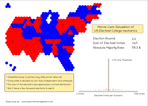
First, but looking the stylized map we see the distribution of electoral votes. Notice that because of our independent and uncorrelated assumption, the distribution of color on the map is really rather random. Yet because there are only two colors and our eyes are always keen to find patterns we easily construct contiguous territories. In fact there is nothing there!

In this particular round the sum of electoral votes achieved by one party is 269, which by pure coincidence is the expected value. The running success rate is 58.3%, far higher than what we might expect, because we only have a very small number of simulations.

Looking the histogram we see that the realizations are quite dispersed and there are only two vote counts that have repeated themselves at this point.

Animating the Simulation Results

We collect all the simulation results in the following video that plays them in sequence. You might want to enlarge the viewing window to see all the detail.

We see that after 1000 simulations the anticipated bell curve is indeed forming (but there is still alot of noise). We notice that the success rate is has drifted below 50% (last reading 48%), but it is by no means stable. This is typical challenge when trying to extract useful information from Monte Carlo simulations: Namely the quantity of interest may not have been estimated to sufficiently high accuracy (has not converged). This can be improved upon with longer simulations or other techniques that reduce simulation noise.

Conclusion

Using simulation in diverse risk management contexts offers rich possibilities to enhance the insight we have into complex systems. This is particularly true when the elements of the system we are interested in are numerous and have potentially complex interactions. Using a simplified version of the rules of the US Electoral College system we illustrated how using Monte Carlo allows us to explore the statistics of the outcomes.