Representing Matrices as JSON Objects: Part 1 - General Considerations
Representing a matrix as a JSON object is a task that appears in many modern data science contexts, in particular when one wants to exchange matrix data online. While there is no universally agreed way to achieve this task in all circumstances, in this series of posts we discuss a number of options and the associated tradeoffs.
Motivation and Objective
Representing a Matrix as a JSON object is a task that appears in many modern data science contexts, in particular when one wants to exchange matrix data online in a portable manner. There is no universally agreed way to achieve this task and various options are available depending on the matrix data characteristics and the programming tools and computational environment one has available.
Matrices are not, in general, native structures in general purpose computing environments. They are rather derived, or composed types, put together from more fundamental types. In most cases they are handled with specialized packages (modules, extensions or libraries). The lack of standardization extends to how they might be represented in computer memory, how they might be accessed programmatically (the API) and how they might be stored in permanent storage. This last topic is of relevance for us here. It comes under the technical term serialization (the process of translating a data structure or object state into a format that can be stored or transmitted.
In this post we will discuss a number of options and associated tradeoffs for serializing matrices into JSON in common programming languages as currently used in data science tasks (such as Python, R, Julia and C++). To make the task finite, we will focus on a subset of possible requirements and considerations:
- The processing speed when serializing / deserializing relatively large matrices from / into computer memory
- The storage requirements when saving large matrices on disk.
- The convenience and ability to represent families of similar matrices
Those metrics serve also as a crude proxy for the speed of transmission of matrix data over the internet (or, similarly, the storage requirements when storing matrices not as standalone files on disks but in databases)
In this first post on the topic we will cover more general ground, defining the concepts and use cases of interest and also initiating a benchmarking exercise. In subsequent posts we will explore additional issues and will go in more depth into specific topics. The cumulative calculations and results will be available in the matrix2json repository on an ongoing basis.
What exactly is a Matrix?
To start with, a Matrix is a versatile mathematical object that shows up in several subfields of mathematics (Linear Algebra, Geometry, Graph Theory and Probability, to name but a few). As part of an applied mathematics toolkit matrices are used in many applications in many scientific and technical disciplines. Matrices are an essential element of many physical theories such as Quantum Mechanics, Optics, Elasticity and Fluid Mechanics. Practical calculations in research and engineering are thus a prime application area. In another broad applications category, the probabilistic interpretation of matrices is the basis for tools such as Markov Chains, which find many applications in economics and finance.
The utility of matrices means that from the earliest days of computing they have been practical implementations to facilitate working with them1. It is worth mentioning here that in computer science matrices are frequently termed 2D Arrays. There is a subtle but important semantic nuance here: using the term matrix instead of array implies that the computational object has additional mathematical properties. Whereas a 2D array can be thought as a bare-bones data container that holds a number of uniform values, a matrix might be expected to satisfy additional constraints or have additional properties in application context. We will return to this distinction below.
The visual appearance of a Matrix is familiar enough: It is a rectangularly shaped array (not necessarily square) or table of numbers, symbols, or expressions (collectively denoted the matrix elements). They are typically arranged in rows and columns, for example something like:
$$ \begin{bmatrix} 10 & 1.2 & -1 \\ 2.1 & 5 & -6.2 \\ -20 & 100 & 0 \end{bmatrix} $$
More generally, we introduce an abstract matrix $A$ as follows: $$ {\bf A} = \begin{bmatrix} a_{11} & a_{12} & a_{13} \\ a_{21} & a_{22} & a_{23} \\ a_{31} & a_{32} & a_{33} \end{bmatrix} $$
The above representation is oriented towards human (and more specifically: visual) perception. The brackets to the left and right of the matrix elements aim to visually enclose the elements and isolate them from other information provided on the page - they have no further meaning (they could also be braces, or other delimiter symbols).
The geometrical layout of the elements $a_{ij}$ on the page (ordered in rows and columns with white space in between) is important in two ways: The up/down and left/right dimensions of the page are used to introduce the concept of columns and rows, while the relative placement (location) of each element assigns implicitly its row and column index.
The actual meaning and usage of these neatly arranged numbers in various domains is the subject of mathematics / science courses, ranging from basic introductions to linear algebra to sophisticated specialized applications in the fields mentioned above. In what follows we will not attempt to summarize all these possible variations, as it would take us too far afield. We will however occasionally reference specific use cases when they might illustrate the practical relevance of representation approaches.
The use context in which a matrix appears determines a number of important attributes for our purposes:
- The matrix size
- The matrix data type
- The matrix density or sparsity
Let’s examine those in turn.
The Matrix Size
The size of the matrix is denoted as N x M where N is the number of rows and M is the number of columns. The special class of square matrices (N x N) appears quite frequently, but we will not need to confine the discussion to this subclass.
The smallest non-trivial matrix dimension is two 2. A matrix of 1 x 1 is a single value (also termed a scalar). The class of 2x2 matrices is already extremely useful in many domains. Small sized 2x2 (and 3x3 matrices) are prevalent in computer graphics and applications related to two and three-dimensional geometries. In quantum mechanics the physics of electrons (Spin) is captured by 2x2 matrices (Paul Matrices). On the other extreme of the size spectrum we have big data type matrices, where the dimension N can reach into the billions.
For our purposes we can informally group matrices by size as follows:
- Very Small size matrices with $N \in [2,3,4]$. For matrices of fixed and low size, such as dimensions two, three or four, the meaning and typical operations on the matrix elements might be implicitly defined by the application context. The classic example would be the two or three-dimensional rotation matrices used in computer graphics and games. Implementations and representations of such matrices will in general be optimised to the application at hand and is outside our scope here.
- Small size matrices with size $3 < N < 20$. This is a domain where each row and column of the matrix may also carry specific relevance and weight. It may, e.g., be a labelled or otherwise distinguishable index (a category label). An example would be e.g., a transition matrix used in financial applications to model credit rating transitions. In this case the size of the matrix is determined by the distinct (labelled) credit rating categories recognized by a rating system. While the size of such matrices would typically not be a concern in modern computers, clear representations and ease of manipulation are becoming important.
- Medium-Sized matrices with size ranging in $20 < N < 1000$. In this size range the individual elements of the matrix are no longer particularly special. They are still individually indexed and identifiable but the expectation would be that they are iterated over programmatically. Examples may be a large Correlation Matrix or a multinational Input-Output Matrix . Efficient representation and working with such matrices is not trivial.
- Large to Very Large sized matrices, with $N > 1000$. An example of such a large object might be the adjacency matrix of a social network (who is connected with whom). This matrix size range enters firmly into the domain of big data. For very large matrices the size itself may be fluidly defined and variable. Working with such data will invariably require very specialized techniques.
The Matrix Data Type
The data type of the matrix elements is in principle flexible. Applications from applied mathematics may involve matrix elements that have a uniform and elementary mathematical type such as integers, real numbers or (occasionally) complex numbers.
Other more complex data types could also be present. Here we will simplify the discussion by focusing only on real numbers (represented either as float or double precision numbers).
In concrete applications the accurate representation of data types might be of extreme importance, in order to avoid, for example, information loss and associated error propagation. The JSON standard that is our target representation format for matrix data is unfortunately not particularly precise about numerical precision 3. Yet, in principle at least, arbitrary numbers could be encoded as strings (and thus preserve all required accuracy), so we leave this complication outside the scope.
The Matrix Density or Sparsity
The density of the matrix is the frequency with which zero elements appear in the matrix. Matrices that feature large numbers (e.g. > 50%) of zeros are termed sparse. Non-sparse matrices are termed dense.4 (or “full”). For large matrices, the density of a matrix may become a critical consideration in terms of both storage requirements and computational performance in calculations. The reason for this is simple enough: The number of elements grows quadratically ($N^2$) if all elements are non-zero, so if $N=1000$ there are a million elements etc. Yet if most of these elements are zero, it may be possible to handle large matrices using specialized techniques. We will revisit issues around sparse matrices in a future post.
To summarize: in the representation of matrices we selected three fundamental matrix attributes, namely Size, Data Type and Density as significant for our purposes. In practice the utility of matrices in applications only becomes realized once we add further features, such as:
- Explicit Constraints on the possible values of matrix elements. These constraints can be simple and directly observable, e.g., we restrict to matrices having only positive values or, matrices that are diagonal, upper or lower triangular or with (anti)symmetric structure.
- Implicit Constraints. Another class of constraints may be “hidden” (or implied) and less immediately visible through inspection of matrix values. For example relations between different matrix values might be required to satisfy some property (e.g. invertible matrices have non-zero determinant, orthogonal matrices have their transpose as inverse etc.)
- Permissible Operations on matrices. The set of meaningful mathematical operations leads to different matrix algebras. There is a vast universe of possible matrix spaces spanned by such operations. For our purposes the prototypical example of matrix operations will be additions and multiplications of matrices (with scalars, vectors and other matrices respectively).
The properties that distinguish matrix objects from “mere” 2D arrays are precisely the facets and attributes of numerical matrix values that are not explicitly captured by the data representations of a matrix. We can think of these properties as a form of metadata about the array values. Such metadate must be communicated separately to convey information as to what precisely is encoded numerically in any particular matrix representation. Another way to think about this is in the context of Object-Oriented Programming. In that context the matrix value would be the data contained in a matrix class whereas the matrix properties would be captured via the class methods.
In-Memory Representations of Matrices
In the previous section we discussed briefly matrices, their types and uses and their human oriented depiction on paper or screen. Now we turn to the representation of matrices inside computer memory.
In computer applications matrices are concrete formations of data (values) that live inside a digital computer’s (RAM) memory. Interestingly enough, conventional computer memory is actually a two-dimensional structure that is laid out as a regular pattern of digital elements on the surface of a silicon chip.
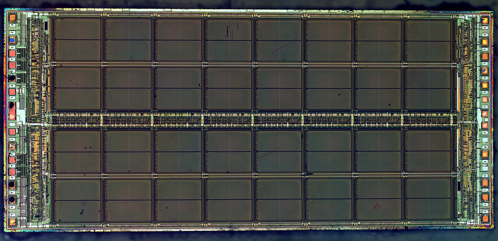
The Physical Memory (RAM) of a digital computer is actually a two-dimensional structure
Yet, despite the underlying geometry, for reasons of simplicity the two-dimensional physical geometry of computer memory is generally not accessible by computer users. Computer memory is addressed instead via linear (sequential), one-dimensional, logical addresses using the computer’s memory management unit. Thus, memory appears to a computer program as a single, continuous address space.
In turn this one-dimensional design of memory access means that some strategy is required when attempting to store composite structures such as matrices (or higher dimensional objects such as tensors).
We will not enter here into the low-level hardware details of how matrix representations are stored in computer memory, but what is important is to appreciate:
- The general approach (for further details see 5 ) of such representations, and
- That the design has can have significant performance implications 6.
Since computer memory is accessed as a linear structure (a one-dimensional address space), a matrix must somehow be “unwound”. To line up all matrix value in a single sequence we must pick one of the two dimensions to start the unwinding process and proceed one row or column at a time until we exhaust all rows or columns:
A matrix is stored in the computer's memory in contiguous (sequential) memory locations as one row following another row, or, as one column following another column. The two options are termed Row-Major Order and Column-Major Order respectively.
The following visualization illustrates this matrix unrolling or flattening strategy:
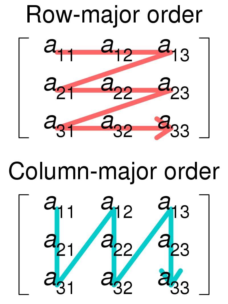
Row and Column Major Order
Hence, if our system uses Row Major Order the matrix would look like the sequence: $$ A = [a_{11}, a_{12}, a_{13}, a_{21}, a_{22}, a_{23}, a_{31}, a_{32}, a_{33}] $$
Similarly, for Column Major Order the representation would be: $$ A = [a_{11}, a_{21}, a_{31}, a_{12}, a_{22}, a_{33}, a_{13}, a_{23}, a_{33}] $$
In high-level languages these alternative representations would in general be hidden by the user but the software might offer them as alternatives via flags or options.
What is JSON and why use it for matrix data?
JSON (acronym from JavaScript Object Notation) is a lightweight data interchange format 7 (compared, e.g., to the more flexible and powerful XML or HDF5 formats). JSON is relatively easy to read by humans (depending of-course on object size and structure) but can also be processed by computers.
As implied by the name, JSON is based on a subset of the JavaScript Programming Language. This has made it the de-facto standard for exchanging data between networked Web applications. The specification of the data format itself is independent of programming language or computer system. The implementation of any associated tools that work with JSON objects will obviously depend on language features (and will inherit, e.g., performance or ease-of-use characteristics from that language).
As JavaScript became the dominant language of client-side web application development, JSON adoption expanded. Being both human-readable and machine-readable JSON moved beyond web pages and is increasingly used in software APIs everywhere. Hence, exchanging various types of quantitative data (including matrix data) in JSON format becomes quite relevant. Alas, the tradeoff of a light specification is that there is no standard way to encode matrices (and arrays more general).
As a starting point, JSON can represent four primitive types:
- strings (sequences of characters)
- numbers
- booleans,
- null (no value)
and two structured types:
- objects and
- arrays
For our purposes we are interested primarily in numbers (and booleans as a limiting case).
Available designs for representing matrices
JSON has two fundamental structures that can be used in matrix representation:
- A collection of name/value pairs. In different programming languages this structure is realized (and called variably as) an object, a record, a struct, a dictionary, a hash table, a keyed list, or an associative array.
- An ordered list of values. Within a programming language environment, this is realized as an array, a vector, a list, or a sequence.
An example key/value pair structure looks like this:
{
  "name":"John",
  "age":31,
  "city":"New York"
}
whereas an array structure involving strings might look like this:
["Chilean", "Argentinean", "Peruvian", "Colombian"]
JSON Representations of Matrices
We turn now to possible choices representing matrices using the above options. The unrolled column and row major orders we discussed above are immediately feasible in JSON using the array element as follows:
["a11", "a12", "a13", "a21", "a22", "a23", "a31", "a32", "a33"]
This representation is pleasantly simple and (presumably) efficient. The challenge is that it does not convey any shape information. The receiver of the matrix data would, in general, have difficulty interpreting it correctly. Is the sequence a square 3x3 matrix or a 2x4 matrix (or maybe a 4x2 one?). This ambiguity can in principle be resolved by constructing a slightly more complex object that adds the missing pieces of shape information:
- An integer value Shape that determines the size of the 1D row or column arrays and
- A binary value Order that takes value 0 or 1 to indicate a row or column order respectively:
{
  "shape" : 3,
  "order" : 0,
  "data" : ["a11", "a12", "a13", "a21", "a22", "a23", "a31", "a32", "a33"]
}
While this augmented representation is a more complete design, it does require that the receiving party recognizes and parses the object as following this particular standard 8.
We turn next to de-facto standards that need less coordination between different users. Good such examples are offered by the structures produced by popular programming environments.
A parametric family of dense matrices
Let us introduce now a concrete matrix that will help us both illustrate concepts and measure performance. Please meet matrix $A(3)$, a small square matrix whose elements span the range 1-9 as follows: $$ A = \begin{bmatrix} 1 & 2 & 3 \\ 4 & 5 & 6 \\ 7 & 8 & 9 \end{bmatrix} $$
A larger sibling of $A(3)$ would be matrix $A(1000)$, a 1000x1000 matrix whose elements span the range 1 to 1 million (for obvious reasons we will not represent this matrix in its entirety!):
$$ A(1000) = \begin{bmatrix} 1 & \ldots & 1000 \\ \ldots & \ldots & \ldots \\ 999001 & \ldots & 1000000 \end{bmatrix} $$
The parametric family of matrices $A(N)$ where $N$ takes any value we choose can be used for benchmarking the performance of different representations. The size $N$ can be made large enough to bring any computing system to its knees! Small scripts that implement and benchmark the different concepts in various languages are available in the matrix2json repository.
Matrix to JSON in the R Language
The most basic data type in the statistical computing system R is the 1D array. The basic array object holds an ordered set of homogeneous values of data type “logical” (booleans), character (strings), “raw” (bytes), numeric (doubles), “complex” (complex numbers with a real and imaginary part), or integers.
The jsonlite package
Using the jsonlite R package9, we get the following JSON representation of an array in row major order.
    library(jsonlite)
    mat <- matrix(1:9, nrow = 3, ncol = 3, byrow=TRUE)
    toJSON(mat, matrix = c("rowmajor"))
which produces:
[
  [1,2,3],
  [4,5,6],
  [7,8,9]
]
We observe that the canonical Row Major Order JSON presentation in jsonlit/R is an array of arrays. NB: We can ask the toJSON function to return a Column Major Order instead:
    library(jsonlite)
    mat <- matrix(1:9, nrow = 3, ncol = 3, byrow=TRUE)
    toJSON(mat, matrix = c("columnmajor"))
The result is another arrangement of values:
[
  [1,4,7],
  [2,5,8],
  [3,6,9]
]
Benchmarking results for R using different JSON packages
We record the following metrics:
- Time to convert (in-memory) a matrix to a json string and save the string to a file (T_out)
- Size of the file (Size)
- Time to load the file and convert it to a matrix (T_in)
For an $A(5000)$ matrix we get the following results for different R packages handling JSON I/O for matrices:
| Package | T_out | T_in | Size |
|---|---|---|---|
| jsonlite | 19.23444 secs | 25.10679 secs | 238.9 MB |
| RJSONIO | 19.62544 secs | 23.94082 secs | 238.9 MB |
| rjson | 4.120749 secs | 16.52509 sec | 238.9 MB |
Notes on the R benchmark
- The file sizes are identical as the format is the same
- Different packages may not preserve the data type
- Recovering the correct matrix orientation in a roundtrip from R to disk and back may require some attention
Matrix to JSON in Python
In python the canonical library for handling arrays and matrices is numpy. While early versions of numpy had an explicit matrix class this is now deprecated in favor of more general nd-arrays.10
[[1, 2, 3],
 [4, 5, 6],
 [7, 8, 9]]
Numpy does not have a direct toJSON function. An intermediate conversion to a Python list is required as follows:
import numpy as np
import json
a = np.arange(1,10).reshape(3,3)
print(json.dumps(a.tolist()))
which produces again the canonical row ordered list format
[
  [1, 2, 3],
  [4, 5, 6],
  [7, 8, 9]
]
For the $A(5000)$ matrix we get the following results for different python packages handling JSON I/O for matrices:
| Package | T_out | T_in | Size |
|---|---|---|---|
| numpy / json | 5.80395 secs | 5.51479 secs | 238.9 MB |
| pandas.to_json | 7.97321 secs | 14.95067 secs | 238.9 MB |
This concludes our first foray into representing matrices as JSON objects and the performance profile of various utilities that allow this type of serialization in R and Python. In the next installment we will focus on a special category of matrices: sparse matrices. Stay tuned!
References
-
Fortran IV: DIMENSION STATEMENT ↩︎
-
When the row or column count is 1 it is more appropriate to talk about an 1D array. When both row and column count is 1 it is a scalar. ↩︎
-
For a more adapted format see Hierarchical Data Format Hierarchical Data Format ↩︎
-
The choice of zero as the element that defines sparsity reflects typical use cases (the underlying matrix algebra). Similar considerations would apply if another element was deemed as carrying “no information”. ↩︎
-
Wikipedia on Matrix Representation ↩︎
-
A program optimization approach motivated by efficient usage of computer memory is termed Data Oriented Design ↩︎
-
The jsonlite Package A Practical and Consistent Mapping Between JSON Data and R Objects ↩︎
-
Numpy Docs: numpy matrix deprecation status ↩︎