Mathematical Representations of Credit Portfolio Data

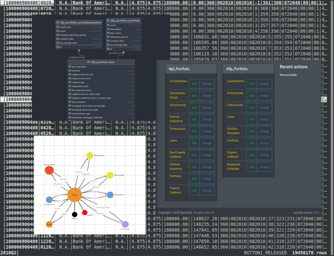
What do we mean by credit data? This post is a discussion around mathematical terminology and concepts that are useful in the context of working with credit data, taking us from network graph representations of credit systems to commonly used reference data sets

Page content

Definition of Credit Data

What do we mean by credit data? For our purposes Credit Data is any well-defined dataset that has direct applications in the assessment of the Credit Risk of an individual or an organization, or, more generally, a dataset that allows the application of data driven Credit Portfolio Management policies. The appearance of credit data is quite familiar to practitioners: A spreadsheet, or a table in a database, with a number of columns and rows full of all sorts of information about borrowers and loans. Digging into the meaning of these data collections, the logic that binds them together, is essential for understanding what they can be used for and what limitations and issues they may be affected by. This post explores a new angle to look at an old practice.

Credit Data

A Credit Portfolio is any collection of credit contracts (Loans or other “Exposures”) that is typically formed as part of financial intermediation activities (e.g., regular lending products offered by banks) but could also be the result of e.g., Trade Finance. Credit portfolios of various sizes and shapes are ubiquitous in modern economies.

The majority of operations that involve credit portfolios are supported by more or less elaborate information technology tools such as: spreadsheets, databases, application programming interfaces and more. Working with such information technology tools requires at least in principle a detailed Data Models , a logical schema about the content, meaning and relationships between different data.

These data models are i) typically proprietary ii) do not address the entire domain in which credit data are collected and updated and iii) are not expressed in concise forms that can be easily perused and understood.

This post is more specifically a discussion around mathematical terminology and related concepts that are useful in the context of working with credit data. While mathematical notation is not a universally understood or practiced tool, it is an important mechanism to convey precise meaning. The objective of this article is to explore in some detail how it can be used in the context of credit data representation.

Caveat: Creating a faithful mathematical representation of credit data will not be an easy task. The implicit context and business logic underlying credit operations (and hence any produced credit data sets) is seldom explicit in data or metadata and is only revealed through concrete usage and practices. When one works with credit data e.g. performing data transformations, creating analytical reports or utilizing credit data to build, e.g., Risk Models one usually injects critical additional assumptions and interpretations that may vary significantly depending on the use case. Nevertheless, we will try to lay an overall canvas and sketch some important principles. The desired result is a small collection of mathematical notation choices that help capture the essence of the credit phenomena one wants to study - as far as those can be captured in concrete data!

Scope and Approach

A top-down (conceptual) approach to our task of expressing credit data in mathematical form might be open-ended and of somewhat limited utility in practical context. We will take a rather narrow slice from this very large domain and adopt a more bottom-up approach that takes into account the (few) examples of actual publicly available credit data schemas. Hence, practically our scope will be guided by publicly available credit data schemas which are explicitly or implicitly documented in portable formats such as spreadsheets or comma separated values (CSV files). More concretely this includes:

In this post we will not go into the details of the above schemas. Interested readers may check out the related Open Risk Academy courses:

One criterion of completeness for our exercise is the degree to which such public schemas can be represented in mathematical notation. A second mechanism to constrain the scope of the discussion is to target expressing well-known operations on credit data. This is, again, a fairly open-ended domain. Such activities are not documented publicly, with some exceptions including academic or regulatory publications. Public methodologies that use credit data typically target the creation of credit risk models, credit portfolio management and valuation of credit contracts etc. Hence, a second criterion of completeness is the number of distinct such operations that can be described using a consistent mathematical notation set.

Further Challenges

Besides the lack of public documentation of credit procedures that generate credit data there are a number of other challenges that we must grapple with. Already the two mentioned examples of actual current credit data dissemination formats hint at some challenges:

  • Different jurisdictions: With jurisdiction differences come significant differences in credit system operations (market structure), contract design, legal definitions around credit events etc. Already within the EU there are important further variations within its member states.
  • Different product scope: The EBA templates cover a wide spectrum of credit products but focus on the non-performing of the lifecycle. In contrast, the Fannie Mae schema focuses on a specific type of single family mortgages, including a wider part of the credit lifecycle.
  • Different adoption stages: US Agencies publish actual historical mortgage data for a few decades already, whereas the EBA NPL template initiative i) is only recently introduced and ii) there are no public disclosures of actual data, only data schemas and iii) it has been subject to significant revisions already.

Yet despite such challenges, there is a substantial commonality of concepts that motivates pursuing the exercise. This commonality ultimately derives from broadly similar business contexts. The ultimate culmination and objective of our exercise will be to have a common mathematical vocabulary for what is sometimes termed a Reference Data Set 1 that is not rigidly tied to concrete credit data but applicable across a range of contexts.

Credit Data Classifications

There is a wide variety of possible credit data depending on the application context. Important classification dimensions include:

  • The information content (the nature of the information captured by credit data)
  • The segmentation by borrower type (different borrowers require potentially very different data sets), or
  • The segmentation by credit product type (again, there is a vast variety of simple or more complex contract which entail credit risk).

It is useful to group these categories into two major types: “hard”, primary or directly relevant credit data and “soft”, secondary or indirectly relevant credit data. Hard credit data are direct and observable reflections of the state of the credit system: they provide an account of what exactly has been legally agreed and is enforceable between the parties involved and how things are progressing over time. Such hard data are not particularly subject to ambiguous interpretations or assumptions.

This group includes data elements such as:

  • Identification Data: e.g., company names or real person identities, business codes, addresses of registered offices, legal forms, dates of establishment.
  • Contractual Data: Namely the details of the credit contract (Loan, Derivative, Lease etc). This will include balances, contractual type, scheduled cash flows, important clauses etc. This category includes contingent contract modification data (in cases where unforessen events lead e.g. to Forbearance measures). Ancillary contracts (e.g.credit insurance) would also be part of this set.
  • Repayment and Servicing Data: The actual track record of credit performance. This includes the recording and representation of any Credit Event that is relevant for the credit relationship and the eventual collection of recovery funds for non-performing contracts.
  • Physical Asset Data: in many instances (mortgages, auto loans, project finance, specialized finance) credit data may capture information about physical assets that are used as collateral (or as part of a lease). In general non-credit data (e.g., geospatial data) will be captured by schemas from other, non-financial domains. An introduction to the use of geospatial data is available at the Open Risk Academy Course: Intro to GeoJSON

Soft, or indirectly relevant credit data are various data points that provide additional insights and context into the performance of the credit system. Soft credit data are generally obtained via longer or more indirect information collection channels and may be subject to more interpretation or assumptions risk. Nevertheless, such credit data are almost always essential for extracting useful information from the entire package. This group includes data elements such as:

  • Accounting and Financial Data: e.g., company accounting records, an individual’s income or asset portfolio.
  • Qualitative Data: E.g., insights from reviews of management structures, client interviews etc.
  • Behavioral Data: Any indicators of behaviors / attitudes that may have bearing on credit performance.
  • Legal History Data: Any judicial track record of Credit History collected from courts.
  • Modelled Data: Data points (such as a Credit Score or Credit Rating ) that are actually composite data, that is derived from a variety of other credit data points.

What is not credit data?

There are several important classes of data that are frequently used together with credit data but do not belong to the credit data category proper. This includes:

  • Macroeconomic variables pertaining to the economic / monetary system (interest rates, exchange rates, economic-wide figures (unemployment, business sector production etc.)
  • Market variables capturing the market based valuation of various commodities or other assets

While at first reading such external data sets are distinct and can be treated as exogenous information sources this might not always a totally benign assumption:

  • Macroeconomic data may already contain various aggregate credit system statistics. There might thus be an in-principle issue of alignment and consistency with more detailed credit data describing a subset of the credit system.
  • Financial markets on credit instruments (e.g., credit derivatives or loan markets) do exist. These provide complementary but possibly also conflicting insights versus purely historical credit data.

Important Aspects of Credit Data we will not discuss

In any practical context Data Quality around credit data is a major concern that may significantly limit the applicability and utility of credit data for decision-making. In this post we will not be concerned with these issues. We assume that the observations of the credit system that we work with are valid. Readers interested in DQ issues may explore the Open Risk Academy Course: Exploratory Risk Data Analysis using Pandas, Seaborn and Statsmodels. Nevertheless, the considerations we explore here do have implications for more abstract levels of Data Integrity Validation (Levels 4 and Level 5) that concern plausibility, completeness or consistency checks between separate domains and distinct entities using the credit data.

From Credit Network Graphs to Reference Data Sets

Credit Provision is a complex business with detailed processes and conventions which determine important data flows and assessments, all within fairly rigid legal and accounting frameworks (Open Risk WP09 2). The mathematical abstractions that are useful in general to describe a credit system include concepts and representations such as:

  • The representation of debtors, lenders and other legal entities involved in a material way in credit relations. These are essentially nodes in a network graph structure.
  • A representation of contractual cash flows (and value exchanges more generally). These can be thought as the edges connecting nodes in the credit graph.
  • Sources of uncertainty that can be modelled as dynamic states that might be either internal to the entities (idiosyncratic) or external (macroeconomic) and linked to global economic system properties.

The last element is of crucial importance and a key reason credit data are collected and processed in the first place: Controlling (managing) sources of uncertainty and the risks and opportunities they generate is core the credit business. Tools used for that purpose are scenarios, namely concrete sets of potential realizations of sources of uncertainty and associated scenario based calculations of asset and liability cash-flows conditional on scenarios, using existing contractual arrangements and assuming the occurrence of potentially unscheduled events.

A general mathematical framework that is conceptually fertile ground for describing credit data is the domain of property graphs (See a previous post and white papers for much more detail and applications around that topic (Open Risk WP08 3, Open Risk WP10 4).

Credit Business Models

The system we want to describe using network graph concepts might be loosely termed a Credit Network , namely an organized credit system where economic entities interact with other entities via credit relations, that is, legally enforceable contractual promises to exchange valuable artifacts over a period of time. We will not repeat here the various elements of graph theory but simply describe the correspondences that take us from a conceptual graph model of the credit system to the reference data set representations used in practice. Very schematically, our journey aims to document the function

$$ \mbox{RDS} = F(\mbox{G}) $$

where $\mbox{RDS}$ is essentially a table of credit data in Long Data Format , whereas $\mbox{G}$ is the (temporal) network graph that offers the underlying abstraction of our credit system.

We are ready now to get started with putting more detail on that canvas, but it is worth repeating that the representation we will sketch is merely a descriptive tool. It does not provide handles for explaining economic phenomena intrinsically (as would, for example be the case with agent-based models that aim to model choices and behaviors of economic actors).

Static Credit Data Snapshots

A basic deficiency of both classic mathematical graph theory and the richer machinery of more recent and application oriented property graphs is that they concern essentially static networks. Given the core objective of credit data to support managing uncertainty, it is essential to incorporate mechanisms to explore alternate possible future outcomes. The mental leap from static graphs to dynamic (temporal) graphs is intuitively not large. Yet while there is an active research field on the structure and properties of temporal graphs, the corresponding terminology, analyses and algorithms are not as mature.

For our purposes the concept of temporal (evolving) credit networks as a sequence of snapshots is already sufficient to provide more concrete mathematical meaning to the term “credit data”.

The problem of representing credit data mathematically is thus naturally split into:

  • the description of the credit system state at a given time point, $\mbox{G}_{t}$
  • the description of the credit system evolution.

From node and edge properties to data tables

Let us start with the first task, a static description at a given time. A key building block of graphs is the set of nodes $V$. Credit graph nodes can be labelled: we can thus distinguish them by their label, which in the simplest case might be just a numerical index. The essential function of nodes is to “hold” information that characterise them. Each node is associated with an attribute vector $[a_1, a_2, \dots, a_n]$. The elements of that vector need not be of homogeneous type or even numerical. The second major building block of a graph are its edges. Mathematically $E \subseteq V \times V$ is a set of edges connecting nodes. Each edge is associated with an attribute vector $[b_1, b_2, …, b_m]$.

What do graph nodes represent? In reality, any concept that appears multiple times in a credit system and can be represented as its own sheet in a spreadsheet or a table in a database. A most natural choice is that nodes represent the uniquely identifiable borrowing and lending entities that participate in the system. Physical assets are also good node candidates. Bilateral loan contracts are good candidates to be represented as graph edges given that they link borrowers and lenders, but can equally well be presented as loan nodes (with an associated Loan ID) and multiple associated properties. We see that the map between the underlying graph of credit relations and tabular credit data is not always straightforward or unique. E.g., One commonly encountered edge case concerns complex borrower structures. In many cases there is just not “one borrower entity” but it is more appropriate to think of a cluster of related entities that are in some way be partially liable for a contract.

Entity Identifiers

Identifiers are typically static credit data that label credit graph nodes or edges. E.g., borrower or loan identifiers identify a unique borrower node or a loan contract respectively. Identifiers are typically alphanumeric in character and range over the set of entities they identify. In mathematical notation precise identities are in general not important. The reason for that is that in much of the downstream use of credit data we assume that entities are representatives of a population. Hence, they can be mapped to integers like: $i \in [1, 2, …, n]$. Subsequently, other credit data can be associated with specific graph entities simply by using identifiers as an index: $A^i, B^{KL}, …, c^{d}$ etc.

A portfolio containing a number of borrowers, loans and collateral might be captured by three data tables:

$$ B^i = [a^i_1, a^i_2, \dots, a^i_n] \\ L^j = [b^j_1, b^j_2, …, b^j_m] \\ C^k = [c^k_1, c^k_2, …, c^k_p] $$

that collect the borrower (B), loan (L) and collateral (C) attributes at a given time $t$ (omitted). The node and edge attributes in the above data tables need not be numbers, only something representable digitally!

In the journey from graphs to data tables and spreadsheets, the labels of nodes and edges become the indices of the corresponding collections of properties.

Composite Variable Names

What does a variable like $a^i_1$ actually mean? Mathematical notation aims to be very concise, reducing representation clutter and focusing on elucidating the important relationships between the various mathematical objects. This leads, for example to represent various mathematical objects with single letters (distinguishing lower and upper-case) and, famously, using also the Greek alphabet to provide additional flexibility. When the discussion happens in a narrow context the single letter approach works fine. But in a credit data context we typically do face a certain difficulty. The number of credit entities and concepts being tracked about them can run into multiple hundreds, so we might run out of letters!

One solution to this problem is the use of acronyms as variable names: E.g., EAD denotes “Exposure at Default”. While somewhat ungainly when used in formulae, the use of acronym-based variables enables addressing a larger domain of entities to be discussed or treated in the same context. The result of adopting this scheme is that our data tables might look something like:

$$ B^i = [\mbox{FTB}^i, \dots, \mbox{AGE}^i] \\ L^j = [\mbox{UPB}^j, …, \mbox{RT}^j] \\ C^k = [\mbox{AR}^k, …, \mbox{MSA}^k] $$

where, e.g. $\mbox{FTB}^i$ is a binary indicator of whether the borrower is a first time buyer.

Qualitative versus Categorical versus Numerical Data

In practice there are three main distinct data types that can be observed in credit data:

  • Qualitative data captured as text. Such data are fairly difficult to use with confidence in quantitative work as the context to which they refer might be very complex. But to a human audience they can be extremely illuminating.
  • Categorical data coded e.g. as integers or some other coding scheme, for example categorical labels identifying things like credit origination channels. Categorical data may be seen as creating subclasses of nodes (or edges), E.g., a boolean flag (First time buyer: Y/N) labels borrower nodes into two categories. A product indicator may signal if a loan is floating or fixed rate. But categorical datea can also be used to represent internal states (more on that below). In contrast to text, categorical data can readily be used in automated procedures.
  • Numerical data which can be integers or real numbers of various sorts. These can further be subdivided into various categories: A credit score is a real number alright, but it has quite distinct qualities from e.g., the nominal amount of a contract. For example, summing up nominal amounts to a portfolio total makes sense but summing up credit scores does not. Numerical data include also some special categories: Dates, pertaining to events and Geospatial Data (coordinates) pertaining to physical aspects of e.g., real estate or the geographic distribution of economic activities.

Correct representation and working with these diverse data types are of extreme importance, especially when persisting (storing) data in various formats or tools. When focusing on purely quantitative work qualitative data are not used, geospatial data are only used within tailored applications and as we will see below, dates are handled in a special way.

A further segmentation that anticipates eventual uses of credit data is the distinction between risk factors (or risk drivers), for example Employment Status and risk outcomes (Credit Default).

A Note on Index Notation

The use of variable indexes ranging over some relevant dimension has an interesting bifurcation of practice in mathematical literature. It is frequently desirable to hide the indexes by using a suitably differentiated symbol for such variables. For example, we might write ${\bf B}$ instead of $B^{i}$ to indicate that there is a concept B (borrowers) which can be indexed by an index $i$ that ranges over some defined range (the set of all borrowers in the portfolio).

The usefulness of such a notational approach rests on the fact that in many areas of mathematics one can represent fundamental operations that involve such objects in concise form. For example

$$ {\bf B} = {\bf B}_{FTB = 1} + {\bf B}_{FTB = 0} $$

might be a way to indicate that the group of borrowers is split into two sets, first time buyers and non-first time buyers. Another example would be to write:

$$ {\bf I} = {\bf UBP} \circ {\bf RT} $$

to indicate that individual elements of unpaid balances and interest rates can be multiplied (on a pair-wise basis) to create a vector of interest income per borrower.

While such “vector approaches” are very convenient and concise when available, they are predicated on certain mathematical (e.g. algebraic) structures being applicable. As you might guess from the variety of data types, that will not generally be the case. A more pedantic but in general more flexible approach is to explicitly track indices of the various dimensions. In our example this would mean writing something like:

$$ I^j = \mbox{UBP}^j \times \mbox{RT}^j \\ I^T = \sum_{j=1}^{N} I^i $$

where the first equation illustrates pair-wise multiplication and second equation uses the summation notation to construct the total interest income.

The explicit indexing approach is not without its own drawbacks. It works, for example, fine when the number of indexed dimensions is small (e.g. up to two or three) but becomes unwieldy as more dimensions get involved - one literally runs out of space to place the indices(!). Indices that are not actively involved in a relation obscure the essence of the operation. One technique that can be adopted to mitigate this is to suppress indices that do not play an important role in a given context.

From Static to Dynamic (Variable) Credit Data

With the machinery we laid out so far we can capture a significant amount of static attributes of the credit system. We turn now to the more complex problem of capturing temporal variability. The general problem in graph terms means phenomena such as the appearance of new nodes in the graph representing e.g., new borrowers, or new edges (representing new lending) or, most commonly, modified properties over time for any of the existing nodes or edges (changing financials, loan amortization through repayment etc.)

Temporal Grids

In practice, due to tractability issues, most representations and calculations involving time-varying credit data are performed in some discrete time framework. This means that a Temporal Grid specifies how precisely the information that describes the state and processes ongoing within the credit system are captured along the temporal dimension.

The temporal resolution of that grid (how closely spaced the observation times) depends on the nature of the credit network and the type of analysis required. Conceptually it must match the timescale on which there is material variability in the credit properties of the system. Observing such variability depends on manifestations such as payments of contractual amounts, accounting reports of financial conditions etc. In general this leads to temporal grids that are monthly or longer. In the simplest case, future cash flows of credit assets and/or liabilities that are part of the overall credit system are considered at a set of given timepoints $t_k \in [T_0, \ldots, T_M]$. When a temporal grid is selected to be more coarse (e.g. annual) all input data must be appropriately mapped or aggregated to fewer timepoints or periods.

Observation Windows

The observation period (window) spans the time interval from some unspecified initial data up to the current date or most recent date. In general the width and location of that window is determined by broader questions around availability, suitability and continuing relevance of historical credit data.

Timestamps and Durations

Contractual data in particular will involve specific periods of time (Loan Maturity, Loan Age, Remaining Life etc.) that are expressed either

  • in absolute terms as temporal intervals $t_k = [T_0,T_M]$
  • in relative terms as the number of periods $T$ over which something happens (e.g., remaining maturity in months)

Contractual (Scheduled) versus Actual Cash flows

Capturing scheduled (or forward-looking) and historical (actual or past) cash flows is a challenging aspect of credit data in that:

  • it concerns lower-level (more detailed) information that is hard to make available as part of loan-level data. This is both because of the higher granularity (e.g. a mortgage loan will involve hundreds of payments) and
  • it involves contingent definitions: amounts might only be determined at future dates on the basis of future observable market variables such as interest rates.

Scheduled Cash Flows

Contractual or scheduled cash flows represent a projection of what cash flows must take place on the basis of the loan documentation. Such projections might be

  • Deterministic and expressed as absolute amounts (e.g. fixed rate mortgages)
  • Contingent and computed in terms of rates and market observables (e.g. floatring rate mortgages)
  • Based on potentially more complex formulas (non-linear expressions involving thresholds such as caps and floors or even more complex logic)

Including complex contractual cash flow specifications alongside credit data is in principle possible but not done in practice. Cash flow schedules are mathematical expressions and as such can be captured in code. Further, since code is data which can be stored and disseminated alongside more traditional data sets one could, in principle, contemplate such combined data exchanges. A concrete proposal illustrates this process using securitisation cash flows.

Schematically, scheduled cash flows for a loan $j$ are represented as a list of temporally ordered functions $\mbox{SCF}_{t}^{j}$:

$$ \mbox{SCF}^{j} = [\mbox{SCF}_{1}^{j}, \ldots, \mbox{SCF}_{n}^{j} ] $$

In simple cases these functions will be mere numbers but, as discussed, in general they are functions evaluating to numbers only at future times $t$. While scheduled cash flows can be indicated mathematically on paper, they cannot be captured concretely in traditional credit data tables.

Actual Cash Flows

Actual cash flows represent a record of what has already happened in terms of value exchanges between borrower and creditor (and any other parties that might be involved in the credit relation). What is done occasionally in order to capture actual cash flow exchanges is to compress select multi-period values as one-dimensional arrays or strings. Schematically, actual cash flows are represented as a list of temporally ordered real number values $\mbox{ACF}_{t}$:

$$ \mbox{ACF}^{j} = [\mbox{ACF}_{1}^{j}, \ldots, \mbox{ACF}_{t}^{j} ] $$

ranging obviously from the start of the credit contract up to the current time $t$.

Discrete Option Exercising Events

In maybe overly reductionist mode we might even argue that managing the deviations between actual cash flows $\mbox{ACF}$ and contractual cash flows $\mbox{SCF}$ is the entire underlying purpose of credit data! The circumstances that can cause such deviations are quite diverse. Excluding extraordinary events such as Force Majeure , in current practices and contracts events signaling important such deviations are typically classified under Prepayment Events, Credit Events or Drawdown Events.

From an economic perspective all the above types of events express the flexibility on the side of the borrower to exercise certain options they legally possess: either i) to repay funds early ii) to not repay funds (facing possible consequences as per applicable law) or iii) to draw additional funds (if legally and practically possible).

Any of these options might be the dominant financial consideration in a particular context. This depends on the type of contract or borrower. Follow-up sequences of additional events may also involve options available to the creditor (for example to seek recoveries by foreclosing on real estate). These can affect cash flows in complicated ways. The manner in which optionality manifests might be captured in contractual clauses (e.g. limits to the amounts of prepayment or drawdowns) but might be also fairly open-ended and contingent on many external actors (as it is the case for example with foreclosure proceedings). We will focus in the remainder on representing credit events.

Identifying and Recording Credit States

A key strategy will be to create credit state indicators. These are defined as indicators (flags) that are built primarily (but not exclusively) by monitoring the deviations between scheduled and actual cash flows. One complication arises from the fact that a borrower may be party to many other credit contracts, the details of which may be unknown to the creditor. Borrower credit performance under these other contracts may affect the credit standing indirectly. For example, a credit default on a separate credit relation may legally make all funds due immediately (hence modify the scheduled cash flows). The implication is that not all credit states derive from directly observable cash flows. At it simplest, though, recording credit states is an indicator of how many payments are past due, which can be counted, e.g. as the number of temporal grid periods.

For long maturity contracts, keeping track on monthly flags might at some point lose its conciseness. For consumer loans a typical coarse segmentation focuses on three distinct states which goes by the following names (naming conventions vary widely by jurisdiction and market segment):

  • Early Arrears Events (up to 90 days past due). During this phase, the focus is on engagement with the borrower to remedy the situation and collect information required for a more detailed assessment of the borrower’s circumstances (e.g. financial position, status of loan documentation, status of collateral, level of cooperation, etc.).
  • Late arrears / Restructuring / Forbearance (90 to 150 days past due). This phase focuses on implementing and formalising restructuring/forbearance arrangements with borrowers. Essentially an amended (modified) contract that aims to be the defining legal document moving forward. From a financial perspective, loan modifications may be classified whether they involve a financial loss or not.
  • Formal Default / Liquidation / Debt Recovery / Legal Cases / Foreclosure / Enforcement. This phase focuses on borrowers for whom no viable forbearance solutions can be found due to the borrower’s financial circumstances or cooperation level. In such cases, creditors typically perform cost-benefit analysis of different liquidation options including in-court and out-of-court procedures.

Besides the duration of delinquency, these three phases are also distinguished by the status of the original loan prospectus: In the first instance it remains in place (but amounts-due continue accumulating), in the second phase the loan gets modified, taking into account events in the first period, while in the final possible stage the scheduled cash flow projections cease to be the driving element (they are still the measure of value that must be recovered) and the focus shifts to any available forms of security (collateral), insurance or credit protection that will be recovered instead of the promised cash flows.

Delinquency Flags

Delinquency flags are constructed by comparing the vector of scheduled and actual cash flows and identifying any discrepancies. A debtor $i$ might be at a time point $k$ assigned (classified) into a delinquent state $S_k^i$ by counting the longest contiguous string of missed payments that ends at $k$. Under such a direct numerical approach the indicator is taking values in $[1,\ldots, M]$ where M is the longest possible delinquency. We might record delinquency status explicitly with binary variables, e.g.,

$$ \mbox{DQ}^i_{t, 30}, \mbox{DQ}^i_{t, 60}, \ldots, \mbox{DQ}^i_{t, 180} $$.

where the numerical figure indicates how many days is the borrower in delinquency. Another way to record that is as a multinomial variable $S_t^i \in [0, 30, \ldots, 180]$

Modification and Default Flags

One can generalize the concept of a credit status flag to include phenomena at advanced stages of delinquency (modifications or default/bankruptcy and liquidation). For example:

  • $M_k^i \in [0, 1]$ might be a modification flag
  • $S_k^i \in [0, 30, \ldots, 180, D]$ is delinquency flag that includes a default state.

An important consideration for credit relationships that enter the difficult zone of forbearance or enforcement is that significant amounts of additional credit data are generated as a consequence. How do those fit into our credit graph and reference data source targets?

The loan modifications undertaken in forbearance activities can be conceptually considered as new loans or more appropriate “loan deltas”. They are thus one or more new nodes with attributes similar to those characterising the original loan. They may also encode any loss amounts that have been written off in these proceedings. For loans that enter the liquidation phase this paradigm is no longer suitable. What happens here is that there are a number of additional costs associated with the proceedings (legal, tax, insurance, asset related costs etc.) and a number of recoveries, on the basis of asset disposals, guarantees or insurance etc. We might represent this as a new contingent node that characterises the liquidation process (e.g., type and timing of court proceedings) and has an associated stream of positive and negative cash flows. All in all our more complete dataset that includes contingent nodes might look like at a future time point $t$ like:

$$ B^i = [\mbox{FTB}^i, \dots, \mbox{AGE}^i] \\ L^j = [\mbox{UPB}^j, …, \mbox{RT}^j] \\ ML^j_1 = [\mbox{UPB}^j_1, …, \mbox{RT}^j_1] \\ ML^j_2 = [\mbox{UPB}^j_2, …, \mbox{RT}^j_2] \\ C^k = [\mbox{AR}^k, …, \mbox{MSA}^k] \\ R^k = [\mbox{FD}^k, …, \mbox{NSP}^k] $$

In the above collection we have in (hopefully obvious notation) a set of modified loan $ML$ entities for every loan $L^j$ that enters such a phase and a set of recovery entities $R^k$ for every collateral $C^k$, with variables like DD and NSP to indicate foreclosure date and net sales proceeds respectively.

Transition Matrices between Credit States

In a sequel post we will explore how the machinery we developed thus far can be used in the context of describing applications of credit data, e.g. in various modeling exercises. As a preview, lets us briefly discuss the concept of a transition matrix that can be readily constructed from temporal credit data.

If we take observations of the credit state variable $S_k^i$ we can perform statistical analysis around the construction of a transition matrix. Namely, estimating the Transition Probability (the probability of moving from credit state m to credit state n) in one time step. Mathematically this is given by $Pr(n|m)=T^{mn}$. The transition matrix $T$ is given by using $T^{mn}$ as the $m^{th}$ row and $n^{th}$ column elements:

$$ P=\left(\begin{matrix} T^{00} & T^{01} & \dots &T^{0n} & \dots & T^{0D} \\ T^{10} & T^{11} & \dots &T^{1n} & \dots & T^{1D} \\ \vdots & \vdots & \ddots &\vdots & \ddots & \vdots \\ T^{m0} & T^{m1} & \dots &T^{mn} & \dots & T^{mD} \\ \vdots & \vdots & \ddots & \vdots& \ddots & \vdots \\ T^{D0} & T^{D1} & \dots & T^{Dn} & \dots & T^{DD}\\ \end{matrix}\right). $$

More information and tools for constructing and working with transition matrices is available in the transitionMatrix library documentation.

References