Portable Standardized Graph Formats for Input-Output Databases

Accessing the wealth of statistical data in Input-Output databases

There are currently several important global initiatives that compile and make available statistical economic input-output data (IO). This is done typically on a multi-regional basis (covering many countries and regions, hence MRIO) reflecting the fact that international trade is (still) very much a reality. Environmentally extended input-output (EEIO) databases that are in turn based on economic activity IO data, are increasingly used to examine environmental footprints of economic activities and play an important role in the attribution and screening of regional and sectoral contributions to environmental stresses.

Yet there is a lot of diversity and complexity in the organization of these typically large datasets. This complicates the adoption and use of EEIO, as it requires the dedication of time and effort to acquire and process data, both initially and potentially with any updates. Motivated by this context, we discuss a simple, generic and portable format for disseminating Input-Output data. The format is inspired from the Graph representation of Input-Output matrices. It allows a unified and very extensible description which can be serialized into standard csv files but also inside a minimal portable sqlite database file.

A cornucopia of Open Data

Even if we only focus on efforts that adopt a free (open data) approach there are several major providers of IO systems. We will refer to them as the different families of IO systems:

• The ADB-MRIO database is the Asian Development Bank’s Multi-Regional Input-Output Tables with a focus on Asian economies
• The EXIOBASE database that has been developed explicitly to address environmental issues
• The FIGARO database (Full International and Global Accounts for Research in Input-Output Analysis) by Eurostat that aims to be the reference IO source for Europe
• The OECD-ICIO database which contains data describing the global economy
• The WIOD (World Input-Output Database) - which is no longer updated (last update 2016)

In addition, large economies may have their own dedicated initiatives: The USEEIO database (US Environmentally-Extended Input-Output is a family of models designed to bridge the gap between traditional economic calculations, and environmental decision-making. There is a corresponding CEEIO database including benchmark IOTs for China since 1990. More specific descriptions for all the above IO families and further links are provided here.

The above indicative list is of essentially independent initiatives, developed over multiple years. It this thus no surprise that the structure and formats used for disseminating the underlying IO data are not compatible. While the logical and mathematical structure of economic IO systems (a set of matrices and vectors with well-defined relations between then) forces a certain similarity of approach and presentation, there are significant variations in how the numerical and explanatory data (labels) are organized and grouped. That diversity extends also into how they are stored in file formats (csv, tsv, xlsx etc.) and/or served via API’s. Together with the fact that IO datasets are typically fairly large (between 100MB and 1GB in size), this creates a practical problem, and (in principle avoidable) frictions, when trying to access and use these valuable datasets.

The challenges with standard matrix representations

The tabular (matrix) representation of IO systems is the most typical form encountered in the above families. It is also the required form once one wants to perform typical IO analyses which involve linear algebra.

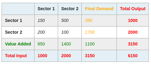
Without going into a full description of the economic IO system logic, the prototypical arrangement of data of an IO system is given by the following diagram that records transactions between different economic accounts. In practice this table would be much larger in size!:

This matrix-like form of the system informs most current approaches of storing and transmitting IO data. NB: There are some exceptions of alternative arrangements, e.g., the FIGARO dataset is also available in so-called flat-file CSV format but the tabular format in general dominates.

The challenge is that a tabular format is not particularly conducive to a clear, uniform, and self-documenting representation. Some aspects causing difficulties, from the more specific towards the more general are the following:

• The data involve a mix of textual elements (labels etc.) and numerical data, in ad-hoc geometries that depend on the size of matrices and vectors (i.e., the number and type of regions and sectors being modeled).
• The large size of multi-regional IO systems (in particularly the large number of columns) make them particularly difficult to load and inspect in tools such as spreadsheets.
• The role of the different data rows and columns is not explicit but is inferred from background knowledge, which varies, depending on how IO systems have been put together.
• There is no clear separation between primary data and derived data (such as control sums)
• Additional complications arise from the fact that many IO systems offer timeseries of data (releases corresponding to different years) which must be loaded and accessed separately.
• It is hard to compare different families of IO systems (from different publishers).

Moving to a graph representation and storage paradigm addresses many of the above issues in a clean way, keeping in mind that working with large datasets does have its own intrinsic challenges that cannot be overcome with simply reshaping how data are organized.

The unifying power of a graph (network) representations

The duality between matrix (linear algebraic) and network (or graph theoretic) representations of IO is well known. We discuss this duality in more detail in the Open Risk Academy course. The graph representation is readily feasible for the classic, symmetric IO systems, and as discussed in the white paper(download) can also be extended to the more fundamental Supply and Use Tables by using a special type of graph (bipartite graphs). This mathematical duality has deep repercussions as explored e.g., in the literature of economic network systems. What we want to focus here is rather more narrow and practical: The possible benefits of representing IO systems as graphs for the purpose of storage and transmission of IO databases.

Let us start with a visual exercise, looking at the graph the corresponds to the above IO table. This looks as follows:

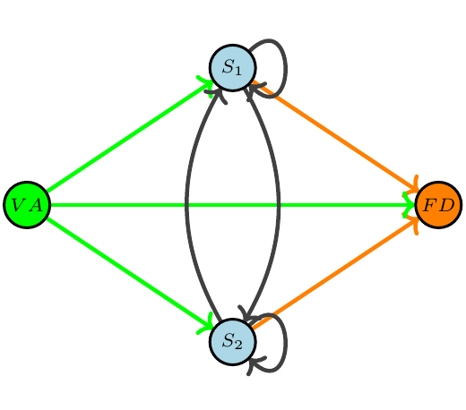
This is a so-called, weighted and directed graph (the weights are the numbers of the table, not shown). A relevant feature for our purposes here is that the final demand column (orange) and the value added row (green) are effectively just another type of graph node (featuring only incoming and outgoing edges respectively).

While the visual representation of a small IO graph may be educational, we are interested in working with large systems featuring thousands on nodes and millions of connections. While there are systems for serializing graph data (DOT, RDF etc) they come with additional specification overhead that may not be needed.

Using tables to represent graphs

A standard representation of an IO Graph utilizes two tables: A graph node properties table that catalogs all available nodes and an edge properties table that does the same for the edges connecting nodes.

The node properties table of our example reads as follows:

Node ID	Node Label	Node Description
1	S1	Sector 1
2	S2	Sector 2
3	FD	Final Demand
4	VD	Value Added

Additional attributes for nodes can easily be added as additional columns. Most typical in Multi-Regional Input-Output systems, one would add an indication of the country or region in which a node operates.

The corresponding edge properties table reads as follows:

From Node ID	To Node ID	Value	Units
1	1	150	EUR
1	2	500	EUR
1	3	350	EUR
2	1	200	EUR
2	2	150	EUR
2	3	1700	EUR
4	1	650	EUR
4	2	1400	EUR
4	3	1100	EUR

Again, we can add useful additional properties per edge (e.g. the units of measurement) without much difficulty. Importantly, we can in this way seamlessly integrate different types of edges between the same nodes (e.g. monetary versus physical unit measurements) without any extra complication.

For example let us imagine that Sector 1 is an agricultural sector producing Paddy Rice and we do have additional measurement information about the volume of trade with Sector 2 (say the Food Processing industry). It is easy to augment the edge properties table with the corresponding measurement, whereas in the matrix representation this is more convoluted.

From Node ID	To Node ID	Value	Units
1	2	500	EUR
1	2	6	Tonnes

Another important flexibility is that one can readily integrate different temporal instances of the IO system, that is, datasets referring to measurements at different periods:

From Node ID	To Node ID	Value	Units	Year
1	2	500	EUR	2015
1	2	550	EUR	2020

In the matrix format each different snapshot can be made available via a different table / file.

Notice that the Total Input / Total Output rows and columns are not represented in the above tables. This is because these sets of IO figures are not nodes or edges, but graph statistics (derived quantities such as column or row sums). Such statistics are useful for validation purposes and can be attached in separate tables.

Practical aspects when storing and transmitting IO data as graphs

A mentioned above, the traditional representation of IO systems as matrix tables utilizes various formats for serialization into files. This then enables transmitting data over the internet. To facilitate such dissemination a common practice is that a diverse set of files (including possibly an entire directory structure) is packaged as a compressed file (zip format etc.). The same options are generally available for the graph representation we discussed here.

Using Files

Standard comma or tab separated formats (csv, tsv) provide the literal encoding of the above two tables (including their headers), so there is not much more to say. A minimal IO system is thus stored simply as a pair of files nodes.csv, edges.csv. In term of size, the first of those files scales with N, the number of nodes, whereas the second file scales with N Squared, the number of possible connections.

It is this second file that will be typically very large as it scales quadratically. Notice that splitting this file in chunks does not create any logical difficulties as there is no implicit order in the arranging of the edge relations and each row is self-documenting. Zipping those files together (potentially with additional textual explanatory notes) is then materializing the entire release.

Another remark here is that graph representations can naturally accommodate sparsity (the presence of many zero values). Effectively only the edge relations that have non-zero values are represented. This does provide some savings in terms of file size.

Using SQLITE as a portable file-based database

An additional advantage of representing IO systems as graph data structures is that it is possible to store even very large systems and even multiple such systems in a conventional relational database. Of particular interest is the use of the lightweight, portable and open source SQLITE database. A key benefit of using SQLITE is that it does not require a database server, with the associated complexities. While accessing data inside an sqlite database does require a dedicated piece of software, such database clients are now generally available. The SQLite file format is stable and cross-platform.

When comparing and contrasting the bundling of graph data into csv files (and a compressed distributable binary) versus the sqlite file option the notable possibility is that the IO data can be accessed and interrogated via standard SQL queries.

A simple, minimalist database schema that can orchestrate persisting multiple different versions of IO systems would involve three tables:

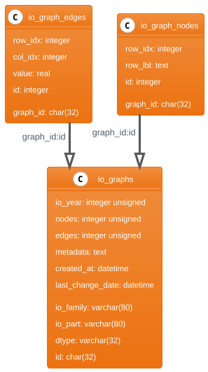
• The IO Graphs table, which serves as the catalog of all possible distinct IO databases stored in the system. This could include e.g. different releases of the same family of IO systems or entirely different families.
• The IO Nodes table stores all the IO node data. It is the database version of the nodes.csv file discussed before. If an IO system offers a time series of data (with uniform regions and sectors), then there is only one such reference table required.
• The IO Edges table that stores all that actual economic transactions datapoints. This will typically be a large table and operations might need to be optimized (with indices) for best performance. As discussed, the edge table format enables significant flexibility to integrate variations of measured data (different epochs, different units etc.)

Of course additional auxiliary tables can be added (e.g., control data for the various accounting balance conditions). This functionality is now being integrated into the Reference app of the Equinox Platform which can be explored online in the Sustainability Town.

Conclusion and Further Work

The representation of diverse public Input-Output databases in graph form (nodes and edges) offers a conceptually clean, practical and extensible way to store such data. Optionally, multiple such IO data sets can be packaged as database tables in a portable sqlite file. In this post we focused on the representation of the basic IO system. In future work we will visit the representation of EEIO data but also the more fundamental SUT representation.