What Can We Learn From Random Walks on Input-Output Tables
In this post we elaborate on the insights we can derive when using well established Environmentally-Extended Input-Output frameworks in a slightly different manner, as the canvas for monetary random walks "following the money"
Summary
We imagine the random propagation of money flows through simplified economic networks as a sequence of monetary transactions following a stochastic process. We follow the journey of a cash amount. Whenever a transaction in this chain implies an environmental impact, that impact is recorded and cumulated. Computing the expected outcome of such flows reproduces the standard results of environmentally extended input-output models. The random walk interpretation allows the computation of various additional statistical properties, one example being estimating a variance of environmental impact or intrinsic uncertainty around the central estimate. We interpret this uncertainty as being a concentration risk measure.
Motivation
The ever growing environmental footprint of complex human economies has raised the need for better tools to understand dependencies and the relative role of economic activities in producing environmental stresses. Such impacts become increasingly threatening to societal welfare and they range from various types of material and water pollution, green house gas emissions, land-use induced biodiversity loss and other ecosystem stresses.
Yet none of these adverse environmental outcomes is the observable and explicitly intended result of a single economic actor. They are typically the side-effect (externalities ) of primary production activities that many find beneficial. The supply chains and networks ultimately creating the impact actually involve a large number of diverse entities. This includes individuals acting both as consumers and employees, producers (companies involving yet another set of individuals), investors, financial intermediaries but also the public sector with various supporting policies, subsidies, guarantees etc.
All these economic actors are transacting across time and space in a complex web. Identifying, quantifying and managing the responsibilities of each actor to incentivise an effective sustainability transition is one of the major challenges of our time, both conceptually and practically.
Brief Review of EEIO Frameworks
One of the most powerful conceptual tools to help with this complex task are the so-called Economic Input-Output Models . These frameworks offer a mechanism to describe an economy in a more holistic way, taking into account these complex interdependencies. For this reason they are currently one of the key tools in analysing environmental impact (alongside more direct measurement methods and the related Life-cycle assessment approach.
The Input-Output concept goes back to earlier centuries and the Tableau economiques of French economist Quesnay. The modern approach of constructing input-output tables and models goes back to the work of Leontief and his famous Leontief Model . This framework has since been elaborated by countless economists and there are now many extensions and variations that are used actively in different contexts.
The essence of an EEIO framework appears deceptively simple: Public sector agencies (such as Eurostat) utilize number of statistical surveys to capture exchanges between economic agents. These are classified and aggregated on the basis of formal attributes such as geographical location, legal entity, business description etc. While there are many processing and reconciliation steps that aim to produce a logically consistent view, the end-result is a directly usable set of IO tables, that record the monetary flows in a from -> to fashion.
By convention the first column of such a table indicates the origin of a transaction while the first row its destination. Transactions can also be within a sector (distinct entities) and those are indicated in the diagonal.
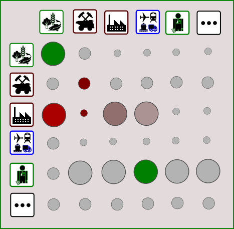
Visual Illustration of an Input-Output system. A number of different Sectors (here six) are shown as both suppliers of goods (leftmost column) and users of goods (first row. The size of the transactions between them is indicated by the size of the corresponding circle, while its impact (positive or negative) is indicated by choice of colors.
Notice that what is being transacted is implicit in the description of a sector, e.g. the Agriculture sector produces and sells “Agriculture”. The number of sectors (also regions - not shown here for simplicity) is quite arbitrary. It depends on the data availability and the objectives of the compiler of the IO database.
Important for our purposes, and already available since decades, the framework has been extended in various manners to account for environmental impact. This has lead to the modern Environmental Input-Output Database . There are by now several such well-developed databases in usage across the world. Constructing a fit for production database that captures the complex global economy in a coherent, actionable, manner requires painstaking work. It involves a large number of assumptions and is subject to significant Data Quality issues. The end result can be considered as an empirical equilibrium representation of an economy. The assumption is that its key organizational structure persists over a period of time that is at least several years.
Modeling potentially changes to that equilibrium is a more controversial but also useful exercise. One of the most typical ways to use EEIO frameworks is to ask: “What happens if demand for certain products or services changes?”. The model produces an answer that takes into account all dependencies between sectors and regions. The value of such EEIO frameworks lies precisely in their ability to capture the interrelationships between sectors in the economy. They help sort out, in a simple and consistent manner, how impacts from intermediate products that are sold from business-to-business cumulate into the total footprint of finished products that reach final consumers.
The Follow the Money Probabilistic Interpretation
The idea of following the money on economic networks such as those imagined in an IO framework is to use a random walk process as a mathematical representation of the fact that funds from purchases or sales of diverse economic actors diffuse through the economic network via financial transactions.
In an economy that is using physical cash (e.g., coins or bills) that diffusion is actually quite literal! Bills will change hands many, many times and the frequency this happens is denoted as the velocity of money . Historically various projects have been setup around the world to track these movements for research purposes.
In modern economies dominated by electronic money that “diffusion” is rather more abstract. It is primarily captured in the set of transactions between private sector bank accounts. Nevertheless, the economic meaning remains the same. Following the travel of a virtual dollar bill from sector to sector, we can trace the origin of funds within an economy or where money is coming from, and the destination of funds with an economy, or where money is going to.
In an open system representation of the economy money comes from final demand sectors (consumption) and ends up to value added sectors. In a closed system money keeps going around, given that consumption is (typically) funded by providing labor services. While the probabilistic interpretation of IO frameworks is not common as it is not required for the classic IO analysis, there are some interesting recent studies: 1 2.
Supply and Use Tables
Taking a step back, one important generalization of the original Input-Output concept is the so-called Supply And Use Framework (SUT). The main idea in SUT approaches is to decouple the notion of a product (a good or service) from the producer entity (e.g. a company within a sector) so as to allow more flexible production structures. This envisions product markets which act as containers for economic production and which all economic entities use to either buy or sell products.
In a white paper we explored how the probabilistic interpretation can be extended to Environmentally-Extended Input-Output frameworks in their Supply and Use Table (SUT) formulation. More specifically we elaborated on the representation of SUT tables as directed, weighted bipartite mathematical graphs and discussed both closed (circular) and open system configurations, featuring source and sink nodes. We outlined a general probabilistic random walk framework that realizes mathematically the colloquial Follow the Money concept in SUT context.
In this post we illustrate the concept using the more straightforward symmetric IO framework and a very simplified IO system.
A Stylized Economy in Input-Output form
We will adopt a popular simple EEIO example3 that has been used in the IO literature for explanatory purposes. It builds a simplified “economy”, in which there are only two producing sectors: Lets call them agriculture (Ag) and manufacturing (Ma) respectively.
In addition there is a household “sector” which will be named Final Demand (FD). This reflects that model has consumers simply buying products as their only economic activity. Of course in reality the economy is closed: households participate directly or indirectly in production in many ways (labor, investments etc.).
There is a special “dummy” sector that represents inflows (Value Added) into the economy. This is not a “real” sector but a place holder for all the inputs would come from some other sector (e.g. households).
Schematically the arrangement is as follows:
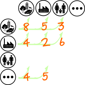
The numbers indicate the volume of transactions between sectors within a defined period (a year). We see the two producing sectors selling goods and services to each other but also to final consumers who purchase the finished products sold by each of the sectors.
More concretely the flow of funds shown indicates:
- The Ag sector purchases \$8 worth of goods and services from other businesses within the Ag sector, as indicated by an arrow pointing from the Ag symbol to itself. Note that the arrows point out the direction of intrinsic value flow (goods or services), whereas the monetary flow is in the reverse direction.
- Businesses in the Ag sector purchase \$4 worth of goods and services from the Ma sector (arrow located in the second row and first column)
- Manufacturing business purchase \$5 worth of goods from Agriculture and \$2 as intra-sector purchases.
- The value-added into the Ag sector is \$4 (third row, first column) etc.
In conventional Input-Output notation this stylized economy can be described using the input-output table as shown below. This is sometimes also called the transactions table.
| Ag | Ma | FD | Total Output | |
|---|---|---|---|---|
| Ag | 8 | 5 | 3 | 16 |
| Ma | 4 | 2 | 6 | 12 |
| VA | 4 | 5 | ||
| Total Input | 16 | 12 |
The table illustrates the annual monetary transactions in the economy and includes also the totals of rows and columns. Again the rows are indexing the from sectors, while columns point to the to sectors, following the flow of goods.
The column labeled FD is the final household demand for the products of a particular sector and the Total Output of a sector is the corresponding row sum. The bottom rows are VA, or value added, and total inputs are correspondingly the column sums. The total inputs into each sector equal the total outputs for that sector. In this simplified economy and financial system the quantity of money is neither created nor destroyed (there are no financial intermediaries such as public or private banks with money creation ability).
Notice that in the standard tabular representation of the IO table the lists of entities appearing on the first row and the first column is not exactly the same. This is for brevity of presentation. The corresponding rows and columns (if we were to represent all entities) would be all zero. We will have to do this below, in order to fully specify the random walk process.
Environmental Impact in the EEIO context
In standard EEIO analysis the environmental impacts associated with the production activities of each sector are assumed to be empirically known (measured). E.g., we assume that a GHG Inventory of the economy has found that activities in the Ag sector resulted in the emission of 8 tons of carbon (per year), and activities in the manufacturing sector correspondingly result in the emission of 4 tons of carbon.
These absolute emissions figures, along with the knowledge of the total output of each sector (the final column of the table), allow us to calculate a direct intensity vector, $f$. This vector gives us the emissions associated with \$1 of output from each sector.
By dividing total production per sector by total impact per sector we obtain that the Ag sector has a direct intensity 0.5 t C/\$ while Ma has a direct intensity of 0.33 t C/\$ ). The direct intensity vector is thus written as:
$$ f = [0.5, \, 0.33] $$
Now we have the very basic machinery of an EEIO table. We will proceed to outline the probabilistic follow the money approach to accounting for environmental impact.
Creating a Stochastic (Transition) Matrix
To proceed with the program we need first to augment the IO table so that all possible “resting points” in the journey of our dollar bill around the economy appear on both rows and columns. In other words we must introduce some empty rows and columns as follows:
| Ag | Ma | FD | VA | |
|---|---|---|---|---|
| Ag | 8 | 5 | 3 | |
| Ma | 4 | 2 | 6 | |
| FD | ||||
| VA | 4 | 5 |
Next, we can proceed to construct a stochastic matrix in two ways: i) by dividing each row value by the corresponding row sum, or ii) by dividing each column by its column sum. Both these options are useful as they emulate different types of random walks. We will discuss briefly both, before focusing on the second approach.
Row Stochastic or Downstream Model
Let us divide all rows values by the row sum (only possible where this sum is non-zero!). We will get:
| Ag | Ma | FD | VA | |
|---|---|---|---|---|
| Ag | 8/16 | 5/16 | 3/16 | |
| Ma | 4/12 | 2/12 | 6/12 | |
| FD | 1 | |||
| VA | 4/9 | 5/9 |
Now each row in this table has become a probability vector (the elements of the row sum to one). No magic, just by construction. This means that starting with any initial sector (any From sector) we have a well defined probability for a transition to any To Sector.
For example there is a $4/12=0.33$ probability that an outflow of product from the Manufacturing sector goes to the Agriculture sector. A similar interpretation applies to all other elements. The special case is the Final Demand sector. Given the postulated nature of this sector (it does not produce any goods), we introduce a unit probability in the third column. This means that if the random walk reaches this sector, it remains there for ever.
Column Stochastic or Upstream Model
Next we derive the column-stochastic transition matrix that we will actually work with more detail below. We divide each element with the column sums (when they are non-zero).
| Ag | Ma | FD | VA | |
|---|---|---|---|---|
| Ag | 8/16 | 5/12 | 3/9 | |
| Ma | 4/16 | 2/12 | 6/9 | |
| FD | ||||
| VA | 4/16 | 5/12 | 1 |
This is a different matrix to what we derived above. The interpretation now is that we can assign a well defined probability for how money is moving upstream, in exchange for products. In other words, the probability that a dollar bill starting from one sector moves to another sector.
In this approach, if the sector we reach along the journey is the Value Added node, the upstream journey is stops permanently. This is expressed by having only a unit probability value in the VA column.
We will denote this matrix with the letter $Q$. For brevity we will use (0, 1, 2, 3) to enumerate the rows and columns (So the Ag sector corresponds to index 0 etc.). We will also be rounding some numbers for simplicity.
| 0 | 1 | 2 | 3 | |
|---|---|---|---|---|
| 0 | 0.5 | 0.42 | 0.33 | 0.0 |
| 1 | 0.25 | 0.17 | 0.67 | 0.0 |
| 2 | 0.0 | 0.0 | 0.0 | 0.0 |
| 3 | 0.25 | 0.41 | 0.0 | 1.0 |
Simulating Random Walks
A random walk over the input-output table can be modeled as Markov chain with probability transition matrix $Q$. The $Q$ matrix is thus the main object we need to construct the random path of a monetary unit around the economic network. We can start the walk anywhere in the economic network by picking a number between 0 and 3 representing the sector we start with. Each different initial condition we pick will probe different aspects of the network.
A discrete-time Markov chain is a sequence of random variables $X(0), X(1), X(2), X(3), \ldots$ where the possible values of the random variable $X$ form a finite set called the state space of the chain. In our case the states of the Markov Chain are in one-to-one correspondence with the sectors of the IO table. The variable $X$ takes integer values in $[0, 3]$, indicating which sector is “occupied” or “visited” at each step of the process.
In our simple example we only have three non-trivial possibilities for a starting sector ($X(0) = 0, 1, 2$). Sector 3 is not relevant since the Value Added sector is an absorbing state. This means we do not learn anything by starting the random walk there.
For concreteness, let us assume that we start in Sector $X(0) = 2$. Thus we will be tracing the money flow from the household sector. The normalized final demand probability column 2 captures which fraction of household outlay goes into which production sector. So for example 0.33% goes to sector 0 (agriculture) while 0.67% goes to sector 1 (manufacturing).
We have selected a value for $X(0)$, how do we obtain the sector $X(1)$ to which the dollar bill will migrate? Simulation of random numbers using a computer program is quite straightforward. We need to draw random numbers from the discrete distribution formed by the probability vector associated with each sector. Clearly to simulate the first step we need to draw a realization for random variable $X(1)$ from the discrete distribution $[0.33, 0.67, 0.0, 0.0]$. Once we do this, we will have a realization of $X(1)$. Conditional on this value we can proceed with the second step. To pursue the full random walk we thus proceed iteratively.
If the draw of $X(1)$ was 0, we draw the next sector $X(2)$ from the distribution $[0.5, 0.25, 0.0, 0.25]$ corresponding to the zero-th index column. In the complementary scenario that the $X(1)$ draw was actually 1, we draw the realization of $X(2)$ instead from the distribution $[0.42, 0.17, 0.0, 0.41]$.
Notice that the realization of $X(2)$ can be 0, 1 or 3, but the probability of it ever becoming 2 (our starting point) is actually zero.
Notice also, that if $X(1) = 0$ or $X(1) = 1$, then it is also possible that $X(2) = 0$ or $X(2) = 1$ respectively. These are transactions where money stays within the same sector (though hopefully not within the same entity).
Finally, both Sectors 0 and 1 have finite probability of leading directly to Sector 3. If the random walk reaches this stage then it must stay there. Operationally this manifests as drawing repeatedly (with 100% probability) the value $X(n)=3$ for all subsequent steps $n$. Obviously in practice we can stop immediately after the first such iteration.
Calculating Environmental Impact along the Random Walk
For environmental impact calculations we’ll be interested in cumulating the impact as the dollar bill travels upstream from consumers to the upstream supply chain. Environmental impact in this simple setup is generated by the buying and selling of products. Of course in reality impact is generated in the production process, not the subsequent trade of products. Yet in the simplified single step approach of input-output frameworks these diverse activities can be packaged into one. In other words, the sale or purchase of a product is instantly associated with the production process of that good or service from the corresponding sector and hence also its environmental impact.
Mathematically environmental impact is obtained for each of the transitions of the random walk, each pair of two successive sectors $(X(t-1), X(t)$ at two successive time steps $(t-1, t)$.
It is common in EEIO impact analysis to consider so-called 1-st, 2-nd etc. rounds of impact. In our context this translates into calculating the expected impact for a sequence of random steps up to the desired number of rounds (which may also be infinite).
In our example, the first transition (from $X(0)=2$ to $X(1)$) would produce 0.5 of impact if $X(1)=0$ and 0.33 if $X(1)=1$.
Here is an example simulation run of a five step “flight” that starts at sector 2 and ends at sector 3 after passing from sectors 0 and 1.
Step 0 : from 2 to 0 with impact 0.5
Step 1 : from 0 to 0 with impact 0.5
Step 2 : from 0 to 1 with impact 0.33
Step 3 : from 1 to 0 with impact 0.5
Step 4 : from 0 to 1 with impact 0.33
Step 5 : from 1 to 3 with impact 0
Running the simulation many times we can calculate the statistical distribution of the environmental impact after any number of steps.
Computing k-round Expectations
In the simplest case we can calculate the expected impact after k rounds using simple analytic formulas. The simplest is the unconditional first round impact. It is simply the weighted average over possible outcomes:
\begin{align} \mathbb{E}(F(1)) = 0.5 * 0.33 + 0.33 * 0.67 = 0.39 \end{align}
Given an initial node $X(0)$, the cumulative environmental impact along a random path up to step $t$ will be the sum:
\begin{align} C(t) = \sum_{s=0}^{t} F(t) \end{align}
While the function $C(t)$ depends on all random variables $X(1), \ldots, X(t)$, the Markov nature of the random process makes the analytic calculation possible.
In the general case we can calculate the expectation of the sum up to $t$ via the following expression:
\begin{align} \mathbb{E}(C(t)) = \sum_k^{t} \mathbb{E}(F(k)) & = \sum_k^{t} f Q^k P(0) \end{align}
where $P(0)$ is the initial probability vector while $Q^k$ is the $k$-th power of the transition matrix.
Example Calculation
As an example calculation, if we explicitly compute the second power of $Q$ we get:
| 0 | 1 | 2 | 3 | |
|---|---|---|---|---|
| 0 | 0.36 | 0.28 | 0.45 | 0.0 |
| 1 | 0.17 | 0.13 | 0.20 | 0.0 |
| 2 | 0.0 | 0.0 | 0.0 | 0.0 |
| 3 | 0.48 | 0.58 | 0.36 | 1.0 |
If we condition on starting with $X(0)=1$ this corresponds to a probability vector $P(0) = [0, 1, 0, 0]$. Doing the matrix-vector multiplications we obtain that
\begin{align} \mathbb{E}(F(2) | X(0)=1 ) = 0.18 \end{align}
The same result is obtained directly via simulation and we can thus validate the accuracy of our Monte Carlo simulation.
Computing k-round Variances
Computing expectations (analytically or via simulations) reproduces the standard EEIO impact attribution, it does not produce any new insights about the economic network. The utility of the probabilistic interpretation is that it allows computing other metrics that follow naturally and which may not be immediately obvious in the standard approach.
The most obvious example of metrics that can be easily built on top of the probabilistic interpretation is a measure of environmental impact variance:
For any round $t$ the definition of the corresponding metric is (as usual):
\begin{align} \mathbb{V}(F(t)) & = \mathbb{E}(F(t)^2) - \mathbb{E}(F(t))^2 \end{align}
In this instance too, we can calculate the statistic analytically as:
\begin{align} \mathbb{V}(F(t)) & = f^2 \circ Q^t \cdot P(0) - (f \circ Q^t \cdot P(0))^2 \end{align}
For the same initial condition as above we get:
\begin{align} \mathbb{V}(F(2) | X(0)=1 ) = 0.05 \end{align}
which means we have a “error” estimate
\begin{align} F(2 | X(0)=1) & \approx \mathbb{E}(F(2 | X(0)=1)) \pm \sqrt{\mathbb{V}(F(2 | X(0)=1))} = 0.18 \pm 0.23 \end{align}
What does this simulated EEIO Uncertainty mean?
Now that we have gotten a taste of how the random walk procedure works and what kind of output it produces in terms of expected impact and variance around that expectation it is high time to ponder: what does this variance (and more generally uncertainty) actually mean? This is an important consideration in deciding how to further use such computations. Let us first discuss some types of uncertainty that our computations are not related to!
An important type of uncertainty in EEIO estimates comes via data quality uncertainties in the underlying data collection and processing. This is a topic that has been studied exhaustively in the Input-Output literature. In related calculations (which frequently involve simulation) the distributions from which one draws alternative realizations are derived from raw empirical dataset characteristics that are used in the construction of the EEIO system. Here we have assumed instead the end-result (the IO table) as given and 100% correct.
Another form of uncertainty is associated with potential intrinsic fluctuations in the economic circulation over time, i.e., a dynamic IO frameworks Capturing such uncertainties would again require access to historical timeseries and more complex model estimates, whereas we have adopted the much simpler equilibrium view.
Yet another type of uncertainty would manifest due to the finite size of actors and their transactions. In an economy where sectors are sparsely populated transactions cannot be considered strictly infinitesimally small. Hence estimates of impact would have an intrinsic variability due to that effect. This is also not our assumption here. We effectively assume that we are operating in a regime where size effects are diversified away and the law of large numbers apply.
The nature of the impact uncertainty implied from a random walk approach derives from the combinatorial aspect of the calculation. Whereas the expected impact is obtained by averaging all possible paths of monetary flows around the economy, uncertainty is estimated by considering the range of alternative possible paths in more detail.
If words, our numerical result that $F(2 | X(0)=1) = 0.18 \pm 0.23$ means that whereas the central estimate of the Manufacturing sector footprint is 0.18, there is an uncertainty around that estimate that is linked to alternative paths in the upstream supply chain of that sector.
Interpreting absolute value estimates of variance is difficult, but relative measures (comparing the uncertainty of different sectors) may be more useful. Absolute values are influenced by the level of EEIO aggregation one adopts to model an economy. This is a rather arbitrary design decision, yet the number of sectors (or regions) strongly influences the outcomes. Instead, in a like-for-like comparison of economies with the same number of sectors will associate higher uncertainty for those featuring sectors with higher impact concentration.
References
-
Carlo Piccardi, Massimo Riccaboni, Lucia Tajoli, and Zhen Zhu. Random walks on the world input–output network. Journal of Complex Networks, 6(2):187–205, 10 2017. ↩︎
-
Olivera Kostoska, Viktor Stojkoski, and Ljupco Kocarev. On the Structure of the World Economy: An Absorbing Markov Chain Approach. Entropy, 22(4), 2020 ↩︎
-
An Introduction to Environmentally-Extended Input-Output Analysis, Justin Kitzes, Resources 2013, 2, 489-503 ↩︎