How Open Data and Open Source can support Green Public Procurement - Part 3
In the third part of this series we illustrate how one may assign greenhouse gas emissions to public procurement using environmentally extended input-output models
Introduction
This is the third in a series of posts where we explore the role of Open Data and Open Source in enabling and accelerating the broad based effort towards Green Public Procurement (GPP). In this third installment we will link procurement entities to private sector sellers and, through the sectoral profile of the procurement contract, (CPV category) we will infer the amount of CO2 emissions that can be attributed to these activities.
Recap of Previous Posts
In the first part of this series we motivated and defined the scope of a study explores Public Procurement data. In the second instalment we dug deeper into an important facet of the data, with the aim of constructing a meaningful economic representation of the public procurement process.
- Part 1 - Overview of the Public Procurement TED dataset
- Part 2 - Identification of Entities involved in procurement
Focusing on Awarded Procurement Contracts
The TED database covers a substantial (but not the entire) part of the public procurement lifecycle1 In our previous posts in this series the analysis was geared more towards the overall activity. Here we focus on the actual awards of procurement contracts. For that purpose we filter all documents from the 2017-2021 period to select forms F03 and F06 (Contract award notice and Contract award notice - utilities respectively). This amounts to 982,794 contracts in total.
Narrowing down the currency universe
As already indicated, the procurement contracts are specified in diverse currencies. For our current sample there are no less than 60 currencies in use! (but many are used rather sparsely). In order to make a proper comparison, we will focus on the most prevalent currencies. We will translate to a common currency (EUR) using a reference exchange rate sourced from the ECB Statistical Data Warehouse2 as standardized SDMX dataflows.
| Currency | Reference Exchange Rate | Count |
|---|---|---|
| GBP | 0.859 | 66397 |
| PLN | 4.565 | 101324 |
| HUF | 358.5 | 12868 |
| CZK | 25.64 | 51910 |
| USD | 1.182 | 977 |
| NOK | 10.16 | 12760 |
| ISK | 150.15 | 502 |
| HRK | 7.52 | 9172 |
| BGN | 1.95 | 39168 |
| SEK | 10.14 | 27177 |
| CHF | 1.08 | 13447 |
| DKK | 7.43 | 9388 |
| RON | 4.92 | 38048 |
| EUR | 1 | 598576 |
Focusing on the main currencies, as indicated above, leaves us with 981,714 awarded contracts where the indicated contract total value is converted into EUR. One final general purpose filter we apply is to remove outlier monetary values. As discussed in the first post, contract values that are either extremely low or extremely large are entered to obfuscate the actual amount being contracted for. A simple way to avoid the serious bias introduced by this unfortunate practice is to remove extreme values3. After we apply this procedure we are left with 889,869 contracts.
Mapping Sectoral Profile
The actual subject of the awarded contract (the precise nature of the goods, services or works to be delivered by the seller to the contracting entity) is not straightforward to identify in the TED dataset. The details will in general be dispersed within the form as verbal descriptions (unstructured data). Further documents with technical criteria, specifications etc. might be outside references that are outside the TED database. The primary mechanism that provides a uniform and easily accessible classification about what product, work or service is the subject of the procurement contract is the CPV classification, to which we turn next.
The Common Procurement Vocabulary
The Common Procurement Vocabulary is the European statistical classification of goods and services procured by the public sector (established by law as the applicable taxonomy to classify tenders). In 1993 the European Commission decided to commence work on drafting its own nomenclature: the CPV system. The use of the CPV codes became mandatory as from 1 February 2006. The most recent version of the CPV is used for publication of tender notices in the Tenders Electronic Daily (TED). The CPV can be traced back to several international nomenclatures used to classify products:
- The Central Product Classification (CPC). This is an international nomenclature developed by the United Nations to monitor world trade. Its main purpose is to provide a general framework for international comparisons of statistics dealing with goods, services and assets, serving also as a guide for other classification systems.
- The International Standard Industrial Classification (ISIC). This is a nomenclature promoted by the United Nations to classify economic activity. Its European counterpart is the European Classification of Economic Activities (NACE)
- The Classification of Products by Activity (CPA). The CPA was developed as a six-digit code system, relating directly to the classification structure of NACE Rev.1 (the first four digits are the same) to provide a product classification for Europe, better suited to European needs.
The CPV consists of a Main Vocabulary and a Supplementary Vocabulary. Both are available in 22 official EU languages. The Main Vocabulary currently consists of about 9454 terms, listing goods, works and services commonly used in public Procurement. The CPV does not offer a structured description for each code. The scope of each term is simply inferred from the string (text) comprising its name and its position in the overall hierarchy. The CPV system is hierarchical with the following overall shape:
- 45 Divisions
- 272 Groups
- 1002 Classes
- 2379 Categories
- 5756 Sub-categories
In this study we will only use the main CPV code of a contract. We also use a mapping of products and services to CPA/NACE sectors to leverage EEIO databases and thus attribute GHG emissions to select components of the procurement portfolio. Let us get on with the task, bearing in mind that it is subject to a number of data and conceptual uncertainties!
Correspondence with CPA/NACE
The correspondence of the CPV with CPA/NACE is not straightforward. Even though they are classification schemes largely following similar economic reasoning the adaptation of the former towards procurement community needs introduces differences. There is a documented mapping between the two systems in4, which nevertheless is
- only partially complete (it utilizes multiple target nomenclatures) and
- is difficult to use as it is embedded in a PDF file5.
For our purposes we only need a high level mapping because EEIO environmental footprint data are only available at such high level. Specifically Level 1 and selectively Level 2 NACE categories. The mapping of the 82 CPV codes is done manually on the basis of descriptions. A fragment is indicated below, while the full mapping is available here
| CPV Code | CPV Description | Exclusions | CPA Code | CPA Description |
|---|---|---|---|---|
| 77 | Agricultural, forestry, horticultural, aquacultural and apicultural services | 772 | CPA_A01 | Products of agriculture, hunting and related services |
| 852 | Veterinary services | CPA_A01 | Products of agriculture, hunting and related services | |
| 03 | Agricultural, farming, fishing, forestry and related products | 034, 0331 | CPA_A01 | Products of agriculture, hunting and related services |
| 772 | Forestry Services | CPA_A02 | Products of forestry, logging and related services | |
| 034 | Forestry and logging products | 341, 343 | CPA_A02 | Products of forestry, logging and related services |
| 0331 | Fish, crustaceans and aquatic products | CPA_A03 | Fish and other fishing products; aquaculture products; support services to fishing | |
| 14 | Mining, basic metals and related products | 147 | CPA_B | Mining and quarrying |
| 15 | Food, beverages, tobacco and related products | CPA_C10-12 | Food, beverages and tobacco products | |
| 18 | Clothing, footwear, luggage articles and accessories | CPA_C13-15 | Textiles, wearing apparel, leather and related products | |
| 19 | Leather and textile fabrics, plastic and rubber materials | 195 | CPA_C13-15 | Textiles, wearing apparel, leather and related products |
Territorial versus Consumption-Βαsed Attribution of GHG Emissions
In common with other domains such (as corporate and financial sector), the attribution of GHG emissions is not unique but may adopt a number of distinct approaches. Each methodology comes with advantages and disadvantages. Information on greenhouse gas and other air emissions can be presented from three complementary perspectives:
- Emissions from the economy from a production perspective (accounts). The production perspective presents greenhouse gas and other air emissions, originating from an economy’s total domestic production of goods and services by different producing entities.
- Emissions from the territory (inventories), which capture environmental pressures that occur within the borders of given jurisdiction / political entity
- Emissions from the economy from a consumption perspective (carbon footprints). This approach focuses on environmental pressure for all goods and services that are finally consumed in an economy along their entire production chain. This point of view is particularly important when goods and services are imported / exported as it accounts for so-called leakage.
Historically the first approach is the so-called territorial approach. It is closely related to the production based approach. This is the attribution of emissions to the entities (and sectors) that are directly responsible for (have most control over sources of emissions) within a geographical region. It is the original conceptual framework as advanced by the IPCC and is thus the basis of national inventories and targets. In terms of the geography of emissions attribution, the territorial approach is most closely aligned with the location of the sources6. On the other hand the consumption-based approach attempts to attribute emissions to the ultimate demand for consumption. Hence, the provision of a final product or service is not attributed only the specific impact associated with a given stage of production, but the entire impact across its supply chain.
Public procurement represents final demand of the public sector, which ultimately provides services to households. The various sectors of the economy thus produce goods and services to satisfy both household demand and public sector demand. Ideally the attribution framework will treat the entire economy consistently. Towards that end we adopt datasets produced by Eurostat as the basis for the attribution7. Specifically, Eurostat produces statistics with a production and consumption perspective and re-publishes the territorial statistics of the European Environmental Agency (EEA). For this exercise we will utilize emissions intensity estimates. Emissions intensities are ratios that assign an amount GHG released per monetary amount. This dataset presents intensity-ratios relating air emissions to economic parameters (value added, production output) for 64 industries (classified by NACE Rev. 2).
Mapping Procurement Sectors to Greenhouse Gas Emissions
While in principle we can mechanically attribute GHG emissions to each individual awarded contract this would not be reflecting correctly the aggregate nature of the Eurostat datasets. Individual contracts (in particular if having specific GPP provisions and criteria) may have an environmental profile that materially deviates from their sectoral average. In such a case the appropriate approach to estimating impact would be, for example, as a GHG Project Protocol that estimates the Business-as-Usual emissions alongside specific, project based reduced emissions from adopting an environmentally friendlier alternative . Clearly such a tailored approach is more data intensive, but is not in-principle incompatible with an allocation based on average profiles.
Grouping the contract portfolio by sector creates 8,216 distinct pools (differentiated also by the five annual periods). As a final simplification to reduce the complexity of further analysis we remove sector / country pools that have low number of contracts (less than two contracts per year). This produces 4,649 pools. We can get a feel by looking at the aggregate top-ten sector / countries combinations in terms of monetary value
| Country | CPA | Value |
|---|---|---|
| FR | F | 157,657,537,681 |
| DE | F | 149,998,869,377 |
| UK | F | 118,447,826,143 |
| PL | F | 61,176,818,348 |
| IT | F | 56,012,553,477 |
| UK | C21 | 5,137,695,4483 |
| IT | C21 | 45,242,868,281 |
| FR | E37-39 | 38,526,298,046 |
| SE | F | 33,757,310,289 |
| UK | M71 | 31,204,444,689 |
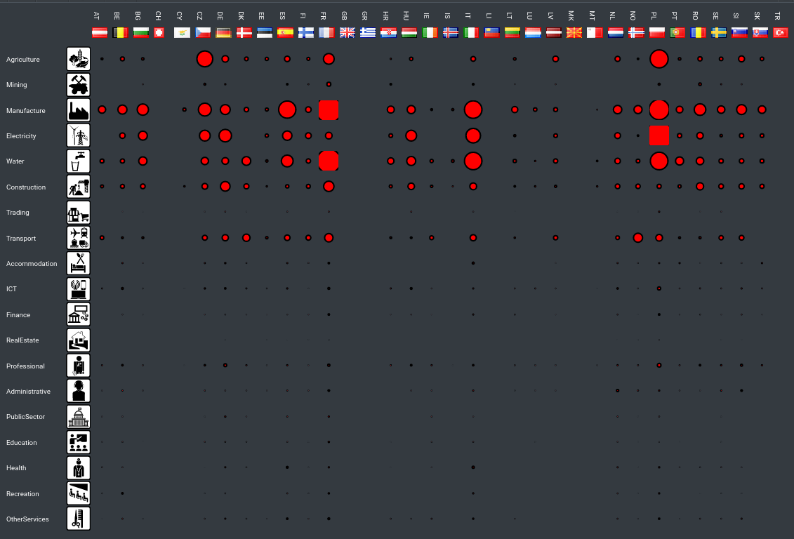
Country by Sector Map of Public Procurement CO2 Emissions
We are now ready to convert the monetary aggregates into equivalent tonnes of CO2 emissions. There is one more detail to take care of: The Eurostat sectoral emissions intensities occasionally are provided also in Level-2 (Division) granularity, such as “E37 to E39” as opposed to simply “E”. For the purpose of a first visualization we will only calculate top-level emissions. With the caveats and assumptions mentioned already we have arrived at the first visual map of public-procurement linked GHG emissions at EU level!
Next Posts in the Series
- Part 4 - Concepts of Portfolio Management in Procurement Context
Open Resources Used
In this section we continue listing various open resources (data, code, standards) that have been used for the discussion (incrementally over previous posts, so as not to produce and repeat excessively long lists)
Open Data
- ECB Statistical Data Warehouse
- Air emissions intensities by NACE Rev. 2 activity
- Eurostat NUTS Notice: © EuroGeographics for NUTS point coordinates
Open Source Tools
Open Standards
- SDMX, a global initiative to improve Statistical Data and Metadata eXchange
Notes and References
-
What is missing are early procurement stages (before notices are published) and the post-award implementation stages. The latter is particularly important for tracking the actual spending under the procurement contract. ↩︎
-
The ECB Statistical Data Warehouse provides features to access, find, compare, download and share the European Central Bank’s published statistical information. ↩︎
-
A slightly more sophisticated Missing Data Imputation would be to look at median sectoral / country values. ↩︎
-
COMMISSION REGULATION (EC) No 213/2008, amending Regulation (EC) No 2195/2002 of the European Parliament and of the Council on the Common Procurement Vocabulary (CPV) and Directives 2004/17/EC and 2004/18/EC ↩︎
-
The linkage to actual sources does not mean that actual measurements are of a physical nature. Most emissions are estimated on the basis of models, assumptions development on the basis of emissions factors and associated measurement of activities (e.g. quantities of fuel burned on expressed in monetary terms) ↩︎
-
Eurostat Air Emissions datasets ↩︎