Mathematical Formulation of Financial Statements

The standard description of financial reporting almost entirely avoids mathematical formulation (variables, equations and using abstraction as a means to step back from less relevant details). While historically there have been efforts to describe the underlying accounting systems in more rigorous language (see ¹, ²), the same does not apply to the higher level of published financial statements. The primary exception is, of-course, the famous balance sheet equation, which, while fundamental, does not remotely cover the richness of of the financial reporting machinery. Our objective in this post is to express the typical financial statements more concisely: using symbolic mathematical notation that substantially captures their numerical information content and the constraints being satisfied.

Why express financial statements using mathematics?

Financial reporting (disclosures) as practiced by various economic entities is a vast domain: several distinct standards are followed across the world and there are multiple special cases within each standard. This is in part addressing the large diversity of accounting entities (from sole proprietors to vast multinationals). There is an overabundance of jargon and conventions, which is ever evolving, in the form of accounting and reporting standard updates that mirror economic and financial system changes. While the avoidance of mathematical formulation ensures accessibility to the widest audience (and is in this sense mandatory towards some purposes), when combined with the large number of quantitative elements and their intricate inter-relationships it also misses the opportunity to provide clear, contained overviews of the underlying mechanics.

In the last decade major progress has taken place towards reporting quantitative non-financial information, further expanding the volume of information being reported. For now these additional disclosures form a disconnected universe that is not easy to reconcile with the corresponding financial representation. Yet as discussed at length in a previews white paper, it is both desirable and feasible to strive to link physical (e.g., environmental impact) and monetary dimensions in underlying accounting systems and external reporting. This integration process requires a clear conceptual and mathematical structure as foundation on which to build practical systems.

Simplifications and work plan

While there are multiple standards and variations of standards we will take a generic IFRS view (and in particular the latest IFRS 18 specification) as a fairly representative blueprint. We imagine a set of statements that is applicable to a generic Small and Medium Enterprise (SME). Depending on accounting context, reporting frameworks may involve a mix of historical cost accounting, accrual accounting and mark to market accounting. While each one of those approaches has mathematical underpinnings, attempting to integrate all of these in one presentation would substantially complicate the discussion. The underlying task requires the mathematical specification of these different measurement approaches, namely the mechanisms for determining the monetary amounts at which the various accounting elements in financial statements are to valued (recognized) and reported (For a sketch of this process see the related discussion in White Paper).

We will thus take an underlying measurement layer that is generating numbers in units of currency as a given. In this context “mathematical” means to represent the relational aspects of financial reporting, namely how these different reported numbers relate to each other. With this focus, the mathematics involved in accounting and financial reporting is actually fairly simple: It revolves around basic arithmetic operations (largely additions and subtractions). Yet the structures built on top these basic operations can be fairly complicated.

The plan will be to express key relations between various reported elements in the financial statements using a set of numerical variables and associated equations. We will ignore any specialized templates for disclosing additional numerical information that might be practiced for specific entities (and of-course any qualitative information that cannot be captured by the monetization paradigm). Before diving into the machinery, let us first name the financial statements that we want to represent.

Note: In general we will not be defining the large number of accounting terms used in practice. Some familiarity with accounting and financial reporting is thus assumed.

The principal financial statements that we will discuss are the following ($ST$ being a shortcut label for each one of the financial statements). :

• ST1: The Statement of financial position (also knows as the balance sheet)
• ST2: The Statement of changes in equity
• ST3: The Statement of comprehensive income
• ST4: The Income statement (also profit and loss)
• ST5: The Statement of cash flows (also flow of funds)

We use the formal IFRS names, though many other labels are used (balance sheet, profit and loss etc.). The chosen order of the statements in the above list is actually important, yet the logic will only transpire later, as we go through the machinery of creating consistent representations.

Some interesting mathematical structures that are implicit in financial statements include the following:

• Categorizations and definitions of aggregate variables. These echo aspects of set theory (but there are only implicit assurances (via audits) of completeness).
• Period-on-period change equations. These expressions link accounting variables between different reporting periods and superficially resemble discrete time differential equations. Importantly though, the causes of change are not modeled explicitly, they derive from the undisclosed underlying accounting system changes.
• Accounting identities that are satisfied by certain subsets of aggregate variables. These are ultimately derived for underlying double-entry bookkeeping system conventions that have explicit mathematical formulations.
• Attribution tables that link various subsets of variables, expressed via linear algebra.

The underlying accounting system as a graph

An important, if maybe obvious, first point is to stress that financial statements are not remotely meant to be the full accounts of an accounting entity. They are merely summary reports, i.e., partial views constructed on the basis of a richer underlying body of data. They are constructed via a sequence of classifications, aggregations and other information processing tasks, from one or more underlying accounting systems, where the measurement processes of tangible and intangible assets, contracts etc. take place.

Similarly to the underlying double-entry bookkeeping, published financial reports must satisfy certain consistency conditions. A word used frequently is that some reported numbers must reconcile. Yet their ultimate faithfulness towards the underlying accounting state of an entity (let alone the actual economic state of said entity!) cannot be established from the financial reports themselves. This assurance is delegated to the role of auditors.

An information model for all the underlying accounting systems is clearly a very complex, if not impossible, task. Here we will assume a simple underlying double-entry bookkeeping (DEB) framework. We imagine an abstract accounting data producing system that feeds accounting values into the financial reports. In the general case this is but an abstraction, but for the simplest accounting entities this may actually be a fairly faithful representation.

We describe the underlying DEB system as an accounting graph (see here for the detailed discussion and examples). Here we will only summarize the most relevant elements for the accounting graph approach. We will not dwell much on the visual aspect of accounting graphs (which is useful for various other purposes) but rather providing concise expressions for transactions and account balances via the concept of a graph incidence matrix.

The accounting graph incidence matrix

The building blocks of the account graph approach to DEB are account modeled as nodes of the graph and transactions modeled as directed weighted edges (arcs) of the graph. There can be multiple transactions linking the same pair of accounts, which is then termed a multi-digraph.

In the accounting graph abstraction, the bulk of the numerical accounting information is captured via a so-called incidence matrix, denoted $b^{ik}$. This is a matrix with the first index $i$ ranging over the number of accounts (say $n$) and the second index $k$ ranging over all transactions (say $m$). An incidence matrix captures all the relationships between accounts and transactions. It is typically represented as follows:

$$ b^{n \times m} = \begin{bmatrix} b^{11} & b^{12} & \dots & b^{1m} \\ b^{21} & b^{22} & \dots & b^{2m} \\ \vdots & \vdots & \ddots & \vdots \\ b^{n1} & b^{n2} & \dots & b^{nm} \end{bmatrix} $$

Each column (each transaction) of this matrix has two non-zero elements: a positive element indicating which account is incremented by the transaction (debited) and a negative element (of exactly the same absolute value, but with reversed sign), indicating which account is reduced (credited) by the same transaction.

As an example, a system with three accounts and three indicative transactions might be: $$ b^{3 \times 3} = \begin{bmatrix} 0 & w^{2} & w^{3} \\ w^{1} & -w^{2} & 0 \\ -w^{1} & 0 & -w^{3} \end{bmatrix} $$

Additional transactions expand the size of the matrix, but the column sum is always zero for all columns.

$$ \sum_{i=1}^{} b^{ik} = 0, \forall k \in [1, m] $$

Visually these graphs are represented as follows:

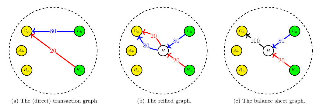
Nodes representing accounts and labeled as Cash, Assets, Liabilities, Kapital etc. are connected by transactions that capture the transfer of value from one account to the other. For detailed calculation examples and correspondences with classic T-account representations check the white paper.

The account balances

A summation over all transactions that connect the same pair of accounts produces the balances of accounts $B^{i}$.

$$ B^{i} = \sum_{k=1}^{m} b^{ik}, \forall i \in [1, n] $$

While at first sight one might think of account balances as properties of nodes rather than edges, in reality they better represented as edge properties. As discussed in more detail in the white paper there are two slightly different graph representations of the same account/transaction set. With the introduction of a central node (so-called reification) this becomes explicit. For our purposes here this nuance is not important.

Since all transactions captured in the $b^{ik}$ matrix balance, the same carries to all account balances $B^{i}$. In other words, the column sum of these account balance vectors is also zero.

$$ \sum_{i=1}^{n} B^{i} = 0 $$

We may think of this equation as the underlying granular balance sheet of the accounting entity. These two numerical objects ($b, B$) are thus the raw material from which we will try to derive the more familiar looking financial statements.

Classification

The familiar labeling of accounts (e.g., as assets, liabilities, equity, income, expenses etc.) is based on shared characteristics of accounts that are always involved (related by) the same types of transactions. E.g. debt type liability accounts would normally have an initial cash flow transaction (the transfer of borrowed amounts from lender to borrower as cash) and subsequent repayments (reverse cash transactions between borrower and lender).

Classification of accounts may focus on the nature, function, measurement basis or any other characteristic of transactions. Mathematically it is a decomposition of the set of accounts and transactions into subsets. In the accounting graph context this amounts to the labeling of the accounting graph elements. Each node or edge can be assigned one or more labels which characterise the nature or function of the account in the contex of the accounting system. Labeling functions (also called indicator functions) map elements of the set of accounts/transactions to specific categorical values.

A first such partitioning exercise is applied to transactions, leading to the labeling of edges(transactions), generated by an indicator function:

$$ \begin{align} 1_{b}(k) & = 1, k \in b \\ 1_{b}(k) & = 0, k \notin b \end{align} $$

The complete incidence matrix can thus be decomposed into a set on sub-matrices that represent categories of transactions.

$$ b^{ik} = \{ b^{ik}_1, \ldots, b^{ik}_b \} $$

This coarse-grained grouping ensures that each granular transaction in set $b^{ik}$ must be included, only once, in some sub-matrix. There is a large variety of possible transactions and enumerating a complete list is not needed for our purposes here. A sample may be informative:

• cash payments or receipts (purchases, sales) in exchange for goods or services
• investments or financing contracts that result in streams of cash flows
• depreciation and other non-cash transactions (revaluations)
• taxation etc.

We can also label and segment the vertical (accounts) dimension of the incidence matrix: For a subset $a$ of the set of nodes (accounts) $i$, the corresponding indicator function $1_{a}$ would be defined as:

$$ \begin{align} 1_{a}(i) & = 1, i \in a \\ 1_{a}(i) & = 0, i \notin a \end{align} $$

Different types of aggregation

Financial statements result from entities processing large numbers of transactions captured in the underlying accounting ledgers etc. Balances in accounts can be consolidated by summing up accounts appearing in the same classification hierarchy (of assets, liabilities, equity, income, expenses etc.). There are many different types of possible aggregations:

• Summing up transactions between the same pair of accounts. E.g. all purchases from the same party. This converts the fundamental multi-digraph into a simpler directed graph, but it does not change the number of nodes.
• Summing up transactions labeled with the same tag by consolidating respective source and target accounts. For example creating a single cash node to represent all cash equivalent nodes.

Using indicator functions we can consolidate transaction impact on account balances, per transaction category with the following summation:

$$ B_{b}^{i} = \sum_{k=1}^{m} 1_{b}(k) b^{ik} = \sum_{k \in b} b^{ik} $$

A vertical segmentation leads us to aggregated stock accounts.

$$ S^{a} = \sum_{i \in a} B^{i} = \sum_{i=1}^{n} \sum_{k=1}^{m} 1_{a}(i) b^{ik} $$

Such variables form one of the cornerstones of the financial statement machinery.

Capturing graph dynamics in coarse-grained fashion

So far we did not say much about the passage of time and how the accounting system evolves. A live accounting system that is accumulating ever more transactions is a formally a type of dynamic graph. While the nodes $n$ of such a graph will typically remain the same over longer periods (major changes to the entity being an example of such fundamental graph changes), new graph edges will be added continuously as a matter of course.

For any realistic accounting system the amount of information encoded in such an ever growing graph structure would be overwhelming to display in raw form. For this reason both internal management systems and external reporting typically present information by introducing various abstractions: Accounting states and transactions are grouped (aggregated) not only according to predefined categorical segmentations and taxonomies, but also over (temporal intervals. A most important aspect of the design of financial reporting in the temporal dimension is the adoption of a stock and flow picture, to which we turn next.

Stocks and flows

An accounting graph representation of the underlying DEB system only knows about nodes (accounts) and edges (transactions). While it is comprehensive and detailed, it does not help with easy interpretation of what is happening. The concept of stocks and flows comes into play when considering the evolution of transactions between accounts over time: As transactions affecting various accounts accumulate, it is natural to group together all transactions occurring over a regular fixed duration, periods, e.g., a set of successive intervals of duration $\Delta T = t_p - t_{p-1}$ which for the majority of financial reporting is customarily an annual period.

The first step in this journey of representation according to temporal order is to introduce the concept of stock and flow accounts. This conceptual tool is common across economics, business, accounting, and mirrors the representation of discrete dynamical systems in natural sciences and engineering. It entails distinguishing between quantities that are representations of state and those that are representation of state changes, or flows.

• Stocks are variables that are measured at a specific time, and represent a quantity (in monetary units) existing at that point in time and having accumulated from past flows (in or out). Stock variables used in financial statements are in general column-wise aggregations. The number of stock variables depicted will in general be much lower than then number of underlying accounts.
• Flow variables are in contrast measured over an interval of time, measured per unit of time. Flows are roughly analogous to the rate of change or speed of a physical system, whereas stocks are analogous to levels or positions. Flow accounts used in financial statements are generated (conceptually) by a sequence of operations: a row-wise sum of select transaction columns that consolidate a set elementary transactions (e.g., multiple purchases of the same type of resource with cash) into one composite transaction column vector and then by column-wise aggregations that reduce the granularity of transaction vectors (e.g., consolidating cash with cash equivalents).

Note: In the accounting literature stock and flow accounts are frequently bundled together under the generic name of accounts. Keeping in mind their different temporal nature helps with understanding the construction of specific financial statements.

Casting the accounting graph picture into a more dynamic setting is quite straightforward: We imagine the incidence matrix starting at some point of time and then augment the matrix by adding ever more columns (balanced transaction vectors) the right of the matrix. This approach mimics a temporal ordering without complicating the notation by keeping track of exact timestamps. We assume we can bucket transactions (edges) appearing within a given period $[t-1, t]$. If the starting balance of all accounts at the beginning of the period, (time $t-1$) is represented by the vector $B_{t-1}^{i}$ and the final balance after a set of intervening transactions $b^{ik}$ during the period $[t-1, t]$ is $B_{t}^{i}$, the following relation links starting and final accounting states:

$$ B_{t}^{i} = \sum_{k=1}^{m} b^{ik} + B_{t-1}^{i}, \forall i \in [1, n] $$

These evolving account vectors are still balancing at all times $t$.

$$ \sum_{i=1}^{n} B_{t}^{i} = 0 . $$

A coarse-grained set of accounts $S^{a}_t$ is constructed by grouping elements from the fine-grained set $B^{i}_t$ by applying a suitable indicator function.

$$ S^{a}_{t} = \sum_{i \in a} B_{t}^{i} = \sum_{i \in a} \sum_{k=1}^{m} b^{ik} + S^{a}_{t-1} $$

This set of equations forms the fundamental building block towards constructing specific financial statements. In words it says that the aggregate evolution of stock variables (assets and liabilities) is the result of the corresponding aggregation of transactions (flows).

When presented with accounts measured at two different periods, the obvious operation is to consider the differences ($\Delta$).

$$ S^{a}_{t} = S^{a}_{t-1} + \Delta S^{a}_{t-1,t} $$

The focus point are the mutations (deltas $\Delta S^{a}$) of the aggregated stock accounts. These are linked to the aggregated transaction flows of each stock account category, which is ultimately linked to the collection of underlying DEB transactions:

$$ \Delta S^{a}_{t-1,t} = \sum_{i \in a} \sum_{k=1}^{m} b^{ik} $$

The next step of the process which leads to actual financial reporting as currently practiced is an ad-hoc selection from aggregated accounting states and associated flows (the set $(S^{a}, \Delta S^{a}_{t-1,t})$, of a smaller number of special interest accounting elements.

The art of constructing financial statements

Up to this point the aggregated system reflects the underlying accounting systems. From this point on accounting convention enters the discussion and somewhat complicates the picture from mathematical point. The parametrized, stock-flow setup of the previous step is not reported as such. Instead financial statements are constructed by reporting a decomposition of specific flows. These choices are ultimately shaped by the requirements of the parties participating in these information disclosure exercises. While in principle any of the aggregated stock accounts appearing in the abstract balance sheet could be explained with dedicated further financial statements (for example, changes in debt liabilities could be disclosed in much larger detail) this typical selection involves a narrower set of stock elements $\hat{S}^{a}$ (with the complement being a less-privileged group denoted $\tilde{S}^{a}$). Correspondingly there are special interest flows $\Delta\hat{S}^{a}$ that explain important accounts and shadow flows $\Delta\tilde{S}^{a}$ that remain unexplained.

As a result of such selections the standard financial reporting equations look (in generic form) as follows:

$$ \begin{align} \sum_a \hat{S}^{a}_{t} + \sum_a \tilde{S}^{a}_{t} = 0, & \text{ Balance Sheet Statement} \\ \hat{S}^{a}_{t} = \hat{S}^{a}_{t-1} + \Delta \hat{S}^{a}_{t-1,t}, & \text{ Select Change Statements} \\ \Delta \hat{S}^{a}_{t-1,t} = \sum_{c \in a} \Delta \hat{S}^{a}_{t-1, t} &, \text{ Select Flow Decompositions} \end{align} $$

In practiced reporting two important types of accounts (equity and cash) are singled out as first among equals and receive their own individual change statements. Let us see what this means in more detail.

ST1: The Balance Sheet (statement of financial position)

Stock accounts appear in $ST1$, the balance sheet. The balance sheet is unique among the five standard statements in that it represents directly all stock account balances that are deemed informative (including those whose changes will not be explained in more detail).

Reporting entities typically classify a number of economic artifacts as assets or liabilities for financial reporting purposes. A sufficient classification for our purposes is the following two-level hierarchy: first a split of stock accounts into abstract assets and liabilities, and then on the one hand into cash-like $C$ and other assets $A$ and on the other side, debt type liabilities $L$ versus equity (capital) type accounts $K$. This produces the decomposition:

$$ S^{a} = \{ \hat{A}, \hat{L} \} = \{ \{ C, A^{c} \}, \{ L, K^{d} \} \} $$

The split into asset and liabilities is mostly a convenient heuristic based on the role an accounting item is expected to play in the economics of the entity. It is not a label that is mathematically rigorous (such as being an account that always has positive measurement value).

Instead of enumerating large numbers of individually named asset and liability types as is done in actual reporting, here will codify the different aggregated accounts appearing in the balance sheet with indices, such as $A^{c}$, $K^{d}$ etc. Various items appearing in $ST1$ are simply summations, like the total value of assets:

$$ A = C + \sum_{c} A^{c} $$

Similarly, there are groupings of reported liabilities that can be aggregated such as:

$$ L = \sum_{d} L^{d} $$

The fundamental balance identity deriving from the underlying DEB system is now recast as:

$$ \begin{align} \sum_a S^{a} & = 0, & \text{ Abstract Balance Sheet} \\ C + \sum_c A^{c} & = \sum_{d} L^{d} + \sum_e K^{e}, & \text{ Expanded Form Balance Sheet} \\ \end{align} $$

ST2: Changes in Equity Statement

As mentioned, one of the indispensable set of accounts that receives royal treatment in standard financial reporting is the equity (net worth, or capital) account, or rather the set of accounts $K^{e}$ that capture the various nuances of the equity interests. Financial reports place significant emphasis on the state and changes to these equity accounts, hinting at who is the primary audience of this knowledge dissemination.

The statement of changes in equity ($ST2$) is a flow type statement that explains the changes in equity accounts induced by transactions. Total (Accounting) Equity $K$ is the amount of residual interest in the assets of the entity after deducting all its liabilities. The $ST2$ statement provides an explanation of changes from the previous period which reconcile to the changes in equity account balances presented in the balance sheet ($ST1$).

$$ \begin{align} K_{t} & = K_{t-1} + \Delta K_t \end{align} $$

Accounting equity is actually a fairly complex element that can be resolved into a collection of the constituent equity components. The equity group of accounts and associated flows of aggregated transactions track new investments or divestment as well as distributions made to shareholders in the form of dividends. The basic equity elements that would be present even in a simple accounting context would be issued capital and retained earnings. A more complete list might include:

• $K^1$, Issued Capital: The nominal value of capital issued
• $K^2$, Share Premium: The amount received from the issuance of the entity’s shares in excess of nominal value
• $K^3$, Treasury Shares: An entity’s own held equity instruments. Treasury shares are not reported as an asset but are subtracted from stockholders’ equity (A so-called Contra Equity Account).
• $K^4$, Reserve Of Exchange Differences On Translation
• $K^5$, Reserve Of Cash Flow Hedges
• $K^6$, Revaluation Surplus
• $K^7$, Retained Earnings: A component of equity representing the entity’s cumulative undistributed earnings or deficit.

The change in total equity derives from the change in individual elements:

$$ \begin{align} \Delta K_t & = \sum_{e} \Delta K^e_t \end{align} $$

This decomposition means that we must explain a collection of changes, in all recognized equity components $\Delta K^e_t$. Towards that end, the statement of changes in equity includes an allocation table. This structure provides a refined picture about where each source of change in equity is attributed to (by which proportion).

The following elements might enter into the change in equity waterfall, starting with the source elements (PnL and OCI, which we will see in more detail later) and the proceeding with increases / decreases due to various actions.

• $CE_0$ = TCI, Total Comprehensive income as the sum of PnL and OCI
• $CE_1$ = Dividends (outflow)
• $CE_2$ = Issue of (new) equity
• $CE_3$ = Owner Contributions
• $CE_4$ = Owner Distributions (outflow)
• $CE_5$ = Equity Other Changes (outflow)
• $CE_6$ = Treasury Share transactions
• $CE_7$ = Ownership interest in subsidiaries
• $CE_8$ = Share based payment transactions

Changes in equity components through the attribution of changes in the various equity elements are represented as follows:

$$ \begin{align} \Delta K^e_t & = \sum_{j} w_{ej} \mbox{CE}_j \end{align} $$

where $w_{cj}$ is an attribution weight matrix (type of charge $j$ versus equity component $e$), with those weights reflecting the exercise of optionality by management and/or investors. Of all the above sources of change in equity, only TCI will be explained further in terms of more elementary flows in statements $ST3$ and $ST4$. The other elements $CE_j$ are aggregations of underlying transactions between various accounts (e.g. dividends) that are not further detailed.

In summary: The change in equity-type accounts is explained as the sum of a number of management/investor decisions and the entity’s economic performance which is captured in a single aggregate flow $TCI$. The further decomposition of $TCI$ is the topic of the next statements, $ST3, ST4$.

ST3: Comprehensive Income Statement

The statement of comprehensive income ($ST3$) is a statement similar in spirit to the income statement $ST4$ that we will discuss below. In one sense it can be considered as a complement to it. It focuses on some items that are excluded from the income statement, but these are items that are required to reconcile (explain) the changes of equity statement $ST2$.

The items in scope of this statement are gains or losses that are fluctuations in the monetary value of assets / liabilities that are not reported in net income. In practice the net income (profit and loss, or PnL) only accounts for earned income and incurred expenses, thus ignores accrued gains or losses that are denoted Other Comprehensive Income (OCI). Mathematically this statement decomposes the change of equity that needs to be explained as follows:

$$ \begin{align} \mbox{TCI}_{t} & = \mbox{PnL}_{t} + \mbox{OCI}_{t} \\ \mbox{OCI}_{t} & = \sum_{k} \mbox{OCI}^{k}_{t} \end{align} $$

Examples of transactions that model unrealized gains or losses aggregated under OCI are:

• Exchange differences on so-called translation (adjustments made to foreign currency transactions)
• Defined Benefit Pension Plans (gains or losses from pension liabilities)
• Revaluation (unrealized gains or losses from debt securities)
• Cash Flow Hedges (gains or losses from derivative instruments)
• Share of other comprehensive income of associates and joint ventures

These flows aggregate nominal transactions between various accounts (e.g revaluation accounts) that typically reflect developments in markets rather than operational actions of the entity itself.

While not as informative of internal operations as the PnL, ultimately it is the statement of comprehensive income that reports the change in net equity and thus reconciles the corresponding equity amounts reported for different periods.

ST4: Statement of Profit or Loss

The income statement $ST2$ aims to provide a more detailed account of the changes to equity caused by entity’s core activities during an accounting period. While the full changes to equity accounts ($TCI$) that reconcile with $ST1$ are actually presented in the Comprehensive Income Statement we just discussed, singling out to explain some of these flows ($PnL$) further in the $ST3$ statement hints that this subset of flows is of particular interest to the users of these reports.

The PnL flow (Net income) is again an aggregation formula bringing together various PnL components $\mbox{PnL}^{k}_{t}$. The PnL aggregates various types of earned income and incurred expenses. It is built as a collection of both cash and non-cash transactions (under accrual accounting).

$$ \mbox{PnL}_{t} = \sum_{k} \mbox{PnL}^{k}_{t} $$

The more detailed PnL component list would be as follows (with positive or negative sign as appropriate):

• $\mbox{PnL}^{0}$: Revenue
• $\mbox{PnL}^{1}$: Cost of Sales (Cost of Goods, Cost of Providing Services)
• $\mbox{PnL}^{2}$: Distribution costs of goods and services.
• $\mbox{PnL}^{3}$: Administrative expenses
• $\mbox{PnL}^{4}$: Finance income
• $\mbox{PnL}^{5}$: Finance costs
• $\mbox{PnL}^{6}$: The entity’s share of the profit (loss) of associates and joint ventures
• $\mbox{PnL}^{7}$: Tax Income (Expense)
• $\mbox{PnL}^{8}$: Profit / Loss from discontinued operations

Revenue ($\mbox{PnL}^{0}$) is a fundamental flow. It is defined as the gross inflow of economic benefits arising in the course of the ordinary activities of an entity when those inflows result in increases in equity. Revenue aggregates positive cash flows (inflows) from transactions that realize some type of value transfer to external parties (sale of goods or services) but it can be realised also with non-cash transactions.

Cost of Sales is another fundamental flow: it is the cumulative negative economic value towards creating sales. It includes transactions for the acquisition of production materials, labor costs paid in cash but also indirect costs that can be directly attributed to generating revenue, for example, depreciation of assets used in the production.

A classification of PnL components that is now mandated under IFRS 18 focuses on the nature of the different components and is split into three major classes:

• Operating Income or Expense
• Income or Expenses from Investments
• Income or Expenses from Financing

which is expressed in the equation:

$$ \begin{align} \mbox{PnL}_{t} & = \mbox{PnL}_{t}^O + \mbox{PnL}_{t}^F + \mbox{PnL}_{t}^I \end{align} $$

With the Income Statement $ST4$ the journey of explaining the change in equity between two successive balance sheets is finally complete! In principle $ST2, ST3$ and $ST4$ are different segments of the same overall statement.

ST5: Cash flow statement

The statement of cash flows ($ST5$) is the last in the sequence of the primary financial statements. It is also a flow statement by structure, but its focus is not the change of equity (a liability account) but rather the change the cash account (an asset). The cash flow statement provides an explanation of changes from the previous period which in principle reconcile the changes in cash accounts presented in the balance sheet ($ST1$).

The cash (monetary assets) of an entity are of special importance for several reasons: they link the company’s economic state (and economic state changes) to the broader monetary system. External transactions are more likely than not to be involving some type of money. Cash (and cash equivalents) provide an important additional lens through which to look at an entity’s economic activities as cash does not suffer from the valuation (measurement) challenges associated will most other assets and liability accounts. In financial terms, cash is simply worth its face (nominal) value, so it provides a measurement basis that is more transparent.

In accounting graph terms the cash flow statement details transactions that affect the Cash account (either have a source or sink into that account), or, more commonly, an aggregated supernode that indicates all highly liquid cash equivalents in whichever form.

The precise structure of this financial disclosure (previously known as the flow of funds statement) depends on applicable accounting standards but in general the changes $\Delta C_t$ in the stock of cash that are detailed in the cash flow statement $ST5$ can be again grouped by type of activity. E.g. under IFRS the decomposition of Operating, Financing and Investing Cashflows is typical.

$$ \begin{align} \Delta C_{t}^O & = \sum_{o} \Delta C_{t}^{o} \\ \Delta C_{t}^F & = \sum_{f} \Delta C_{t}^{f} \\ \Delta C_{t}^I & = \sum_{i} \Delta C_{t}^{i} \end{align} $$

$$ \begin{align} \Delta C_{t} & = \Delta C_{t}^O + \Delta C_{t}^F + \Delta C_{t}^I \\ C_{t} & = C_{t-1} + \Delta C_t \end{align} $$

Putting it all together

We are now in a position to put all the pieces together in a simple collection of variables and equations. The overall structure of the financial statements can be summarized now as follows: Aggregated stock accounts appear in $ST1$. Of all the recognized stock accounts, equity and cash type account flows are explained in $(ST2, ST3, ST4)$ and $ST5$ respectively. Thus changes to equity are reported in a hierarchy with three levels (though in principle it could all be done in one change of equity statement).

Statement Hierarchy

Stock Accounts at t-1, t	Flow Accounts (L1)	Flow Accounts (L2)	Flow Accounts (L3)
$ST1$ (Financial Position)
$K_t$ (Equity)	$ST2$ (Changes in Equity)	$ST3$ (Comprehensive Income)	$ST4$ (Income Statement)
$C_t$ (Cash)	$ST5$ (Cash Flow Statement)

Aggregated Relations

$$ \begin{align} K_{t} & = A_{t} + C_{t} - L_{t} & ST1 \\ K_{t-1} & = A_{t-1} + C_{t-1} - L_{t-1} & ST1 \\ \Delta K_t & = w_0 \mbox{TCI}_{t} + \sum_e \sum_j w_{ej} \mbox{CE}_j & ST2 \\ \mbox{TCI}_{t} & = \mbox{PnL}_{t} + \mbox{OCI}_{t} & ST3 \\ \mbox{OCI}_{t} & = \sum_{k} \mbox{OCI}^{k}_{t} & ST3 \\ \mbox{PnL}_{t} & = \sum_{k} \mbox{PnL}^{k}_{t} & ST4 \\ \Delta C_{t} & = \sum_{a} \Delta C^{a} & ST5 \\ \end{align} $$

Linkage with Graph Incidence Matrix

$$ \begin{align} S^{a}_{t} & = \{ \{ C_{t}, A_{t} \}, \{ L_{t}, K_{t} \} \} \\ S^{a}_{t} & = \sum_{i \in a} \sum_{k=1}^{m} b^{ik} + S^{a}_{t-1} \end{align} $$

Conclusions

• The machinery of accounting graphs is quite powerful: using the incidence matrix it is possible to construct higher level abstractions such as those found in financial statements
• The balance sheet identities derive directly from the underlying DEB structure. Other reconciliations found in financial statements are only establishing correspondences between statements.
• The number and structure of financial statements is discretionary. In principle there are only two statements: a stock and a flow statement.
• The focus of conventional financial reporting is on explaining equity and cash flows. A more integrated sustainability reporting framework may motivate isolating further accounts (e.g., those with material impacts) to provide a more holistic report of changes.