Methodologies for estimating data center environmental impacts

In the first post of a series dedicated to the measurement of data center environmental footprints we reviewed the conceptual thought frameworks and challenges. The main objective in this second post is to outline current measurement methodologies and document their quantitative prescriptions in mathematical form.

While the post can be read on its own, various terminologies and concepts that are useful have been explained in the first post and will not be repeated here.

The objective of environmental impact measurement methodologies is to compile and disseminate to stakeholders useful environmental impact metrics. These metrics are generally quantitative: they are numerical indicators, possibly in defined physical units. In the first post of this series we listed the broad list of impacts that are being discussed in the context of data center environmental footprints. Here we focus on two of these impacts, namely carbon and water footprints, as these two metrics are currently investigated and reported as the most relevant. The corresponding numerical indicators will be notated as:

• $I_{g}$, standing for the volume of GHG emissions of a datacenter
• $I_{w}$, representing the volume of Water consumption

Both of those environmental stresses are in reality complex clusters of more detailed phenomena:

• Emissions concern a variety of different green house gases, which for simplicity in general practice are converted into tonnes of CO2 equivalents.
• Water usage is also subject to further distinctions: concerning the type of water used, such as blue water extracted from rivers, lakes and groundwater, grey water reuse, the condition of any water returned to the ecosystem etc.

Data center related economic activities might have both direct and indirect environmental impacts. Indirect impacts are these generated, e.g., in the construction of data centers and IT equipment, or associated with end-of-life disposals, or the downstream use of their digital services by clients and end-users. Our focus here will be narrower, on the environmental impact from data center operations, the activities during the use-stage of IT equipment when providing digital services to external users. In the GHG Protocol context and terminology¹ this means that the Scopes of interest here are Scope 1 (the direct, or on-site impacts) and Scope 2 (the indirect impacts through purchased electricity). We can capture the respective split for both types of impacts as follows:

$$ \begin{align} \begin{bmatrix} I_{g} \\ I_{w} \end{bmatrix} & = \begin{bmatrix} I_{1,g} + I_{2,g} \\ I_{1,w} + I_{2,w} \end{bmatrix} \end{align} $$

where the indices in indicators $I_{1/2,g/w}$ suggest the impacts concern Scope 1 or Scope 2, and GHG emissions or Water Use respectively.

Measurement approaches

The objective of measurement methodologies is to link these four estimates to available data.

It is methodologically important (and not true for other impacts) that these two environmental impact indicators ($I_{g}, I_{w}$) are closely related to the operational energy consumption of the IT and non-IT equipment of the data center.

Using operational energy as the common underlying driver for both emissions and water usage will allow us a small simplification that we will highlight. As counterexamples, there are important impacts associated with data centers, such as the embodied impact in manufacturing the IT equipment, end-of-life e-waste, and other environmental and social implications (e.g. land use) that are not strongly linked to the operational energy consumption.

Owners and/or operators of data centers have in principle access to a wide variety of inventory and operational data that can help analyse environmental impacts:

• Data center specifications and designs (total area, density, non-IT technologies used)
• IT equipment inventories, including their types, costs, power characteristics, number of servers etc.
• Energy and water provision contractual arrangements with utilities.
• Directly metered data for electricity and water use.
• Financial transactions (payments) for electricity and water use.
• Operational statistics (telemetry) for the utilization rates of both IT and non-IT equipment.
• Data about on-site energy generation (gas turbines, backup diesel generators etc).

In paper² a comprehensive list of metrics and KPI’s at various levels, from facility to IT component is enumerated, but in general only a very small fraction of the above list will be publicly disclosed.Operational activities are in turn linked in non-trivial ways to the external demand for digital services. The nature and volume of externally provided digital services is another potentially important data input, but it is considerably more fraught with complexities, so we leave it out of scope.

Direct and indirect measurement

Environmental impact data (in our case GHG emissions and water usage) can conceptually be gathered in one of two ways: direct, at the source where the impact is generated or indirect, from once-removed but still causally linked information flows.

• Directly measured means that the environmental impact of data center processes is quantified from on-site measurement devices (sensors, meters etc.). For GHG emissions, such direct measured data points, e.g., from sensors, while possible using greenhouse gas monitoring infrastructure this is in general not available. In contrast, for water use, the direct metering of consumption would be the norm.
• Indirectly measured (or modeled) means that the quantification relies on other information flows. The most common case is the recording or modeling of process activity data, along with corresponding emission factors or intensities.
  • Activity data are extensive variables that quantify the magnitude of operational activities within the data center, in absolute terms. In turn such data indicate the volume of GHG emissions or water consumption happening within the data center or its environs.
  • Intensity data will provide energy or power consumed per unit of activity. Eventually they indicate GHG emissions or water use per unit of energy consumption activities.

Activity data, when combined with different types of intensity data, result in the indirect calculations of energy and GHG emissions or water usage. Activity data and intensities are always paired. Individually they do not provide complete information.

This methodological decomposition on the one hand provides alternative data sources, on the other it opens up the possibility of what if analysis. This is done by projecting alternative scenarios either for technology driven factors or demand driven activity or both.

Further, it is useful to use the GHG Protocol³ nomenclature of primary vs secondary data to classify different methodologies for estimating energy consumption (and thus impact).

Primary, secondary and proxy data

Primary data come from any process activity that directly captures the electricity consumption of the inventory (IT and non-IT equipment). Examples of such primary data include:

• Metered electric power or energy (e.g., MWh of energy drawn from the electric grid).
• Lapsed time (e.g., hours of operation of IT equipment or CPU time at average power draw).
• Mass (e.g., kilograms of fuel burned in purpose-built gas plants or other on-site power generation).
• Equipment inventories, including counts and types of servers etc.

Under the GHG protocol using primary data is required for reporting emissions that are under a reporting company’s ownership or control (Scope 1 emissions). But there are potentially data sources that are less specifically linked to the energy consumption and environmental impact of any given data center. These are termed secondary data. Secondary data can come from a variety of sources. Most typically these will be external source (e.g., industry average data).

Finally, proxy data refer to another process or activity that is causally related, but is not identical with the activity driving the environmental impact. Proxy data might include a variety of physical or financial metrics such as:

• Data center floor area. This is a frequently used metric as a simple proxy for Data Center Capacity.
• Other operational metrics: Average GFlops, GB volumes of data stored, volumes of GB data transmitted over networks etc.
• The monetary value of digital services provided

For proxy metrics to be useful, they must still reflect faithfully the data center energy use and, ultimately, environmental impacts. Being less directly related with a data center’s operational activities, they may be affected by additional drivers or factors, which might dilute the relationship to energy usage, introduce biases etc. Proxy data may also be incomplete in terms of scope, due to imperfect overlap with the inventory of impact sources within the data center.

We can organize all the above in a table:

Measurement Type	Energy Usage	GHG Emissions	Water Usage
Direct (measured with sensors, meters)	Yes	No	Yes
Indirect (modeled)
- Primary Data	Inventory, Utilization	Energy Usage	Energy Usage
- Secondary Data	Average estimates per data center type etc.
- Proxy Data	Floor space, financials, service volumes etc.

The table splits out energy usage in a distinct column, in addition to two target environmental impacts. Besides being a data input, energy usage is an important data point in itself, in terms of the demands on local grids and thus other stakeholders depending on energy utilities.

If proxy and secondary data are available in addition to primary data, it creates a luxury problem. They can be used to double-check and probe the overall consistency of impact estimates, identify outliers etc.

Basics of Data Center Energy Consumption

Before we dive into the main methodological approaches, it is useful to establish some notation and terminology around data center energy consumption. Data center capacity is a somewhat loose term that ultimately aims to indicate the volume of digital services that a facility can provide, e.g. how many commercial entities or households it might support. In its most concrete form capacity is measured in terms of provisioned electric power.¹ In terms of units, electric power is measured in watts (W) or multiples thereof: kilowatts (kW), Gigawatts (GW) etc. The order of magnitude that is typical for data centers is the Megawatt (MW). Indicatively, total data center capacity as reported by IEA⁴ has grown from 20 GW in 2005 to 100 GW in 2024. Having a reasonably accurate indication of a data center’s capacity is an essential data point in estimating environmental impacts.

Correspondingly, energy consumption will be measured in watt-hours (Wh), kilowatt-hours (kWh) etc. The total energy consumption reported by IEA has grown from 150 TWh in 2005 to more than 400 TWh in 2024. The fundamental power-energy relationship is that the total energy consumed within the perimeter of data center ($E_{dc}$) equals the total power consumption ($P_{dc}$) multiplied by the measurement or observation window (T).

$$ E_{dc} = P_{dc} \, T $$

The time interval T that is typical for sustainability reporting purposes is annual, which coincides with the financial reporting cycle of major corporations. As an example, dividing the above reported IEA energy consumption py the corresponding capacity estimate we get:

$$ \frac{400 \, TWh}{100 \, GW} = \frac{400 \, 10^{12}}{100 \, 10^{9}} h = 4000 \, h $$

which indicates that the data centers included in these estimates were operating at roughly 45% capacity.

How is energy demand satisfied

Data centers can be powered both by local sources (on-site) and via electric grid connections. On-site energy production, also called behind-the-meter (using e.g., diesel or gas) was traditionally used as a backup energy generator or when grid power is not available.⁵ The majority of energy currently used is source from the local electric grid, yet grid capacity constraints means there are scenarios of significant behind-the-meter, on-site energy generation going forward. We therefore decompose total energy supply into on-site and grid electricity respectively:

$$ E_{dc} = E_{os} + E_{gr} $$

These can be expressed as fractions ($\lambda$) of total energy supply:

$$ \begin{align} E_{gr} & = \lambda E_{dc} \\ E_{os} & = (1 - \lambda) E_{dc} \end{align} $$

With this decomposition we can in-principle address impact intensity differences between grid and on-site generation.

Handling demand variability

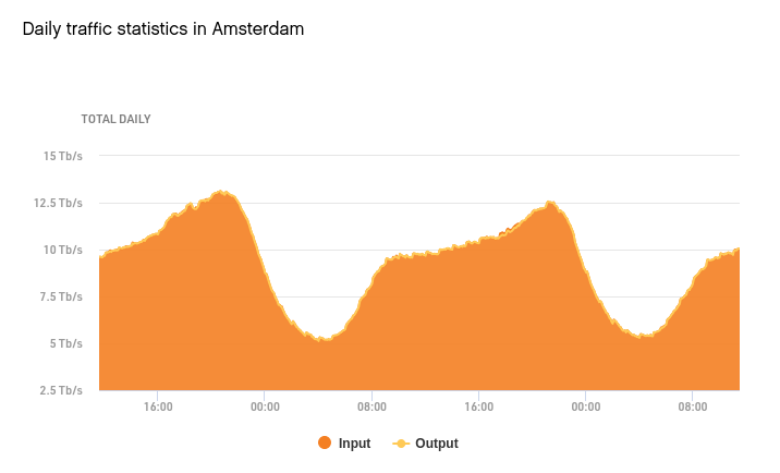
The assumption in the above equations is that power consumption is constant. In reality the power drawn by a data center is anything but constant: over a year it will vary continuously, depending on the type of services it provides and other circumstances.

When handling a variable power envelope, in the most detailed case one must work with the integral of power over time.⁶

$$ E_{dc} = \int_{0}^{T} P_{dc}(t) dt $$

Yet this level of detailed analysis is only realistic for internal data center use cases, and low-level modeling. For basic environmental estimates of average power is sufficient. In practice certain power related parameters capture the essential aspects of variable power consumption profiles⁷. Here is a small such list:

• Rated power: this is the absolute maximum possible power draw of the IT equipment, as obtained e.g., from the specification sheet.
• Maximum power: $P_{max}$ is the measured power draw when the equipment is operating at its maximum workload. In general this will be lower than rated power.
• Operational power: this is the measured power draw when the equipment is operating in a typical workload mode. This is assuming such a typical workload exists!
• Idle power: $P_{i}$ is the power draw when a equipment is sitting idle (thus it is the minimum power, when not processing any useful tasks)
• Average power $P_{a}$: is the measured average power drawn over a period of time. This the quantity we are eventually interested in.

The motivation to dwell on the variety of standardized representations of variable power consumption is for inferring average power when it is not directly available.

A data center will typically be designed to a specification of the maximum power provisioned to the IT component. So when there is talk of, e.g., a new 100 MW data center, this sketches a facility that will be able to support IT equipment that, in toto, draws up to this amount when operating at maximum power. The necessary non-IT infrastructure equipment to support 100 MW of power, cooling capability etc. is aligned with this maximum power (See PUE below). If the maximum power provision is known, we might be able adjust it for obtaining an estimate of average power, but we will need additional data. Or we can proceed to compute environmental impact estimates on a conservative basis, as an overestimate.

The average power drawn by IT equipment can be expressed as the interpolation between maximum and minimum:

$$ P_a = u P_{max} + (1 - u) P_{i} $$

where $u$ is the average utilization rate or load factor of IT equipment. When the load factor is 100%, the power consumed is $P_{max}$. When the load factor is 0% the power consumed is $P_{i}$. Smaller data centres might have average utilisation rates below 20%, while large data centres with optimised workloads can have average utilisation rates above 50% ⁴.

An alternative expression⁷ is the following: if the power curve is well presented by an operational period $T_o$ and an idle period $T_i$, we have

$$ P_a = P_{o} \frac{T_o}{T} + P_{i} \frac{T_i}{T} $$

where $T = T_o + T_i$ is the total observation period.

IT versus non-IT power demand

The total data center power draw is considered to be the sum of the power drawn by the IT and non-IT components respectively. As mentioned, a data center will in general use more input energy than what is delivered to the IT equipment that provides the desired digital services. We can decompose this split as:

$$ P_{dc} = P_{it} + P_{nit} $$

or in energy terms

$$ E_{dc} = E_{it} + E_{nit} $$

The IT component itself includes different equipment such as Servers, Storage and Networks. Further, each of these technologies may come with their own subcategories, each with different power characteristics. For example, CPU servers versus GPU accelerators have different power draw requirements. Data center CPU servers in 2025 had an average thermal design power (TDP) rating between 150 watts and 350 watts. In comparison, a data center GPU can have a maximum TDP rating between 350 and 700 watts. Similarly, different vintages of CPU’s or different architectures may have markedly different power demands. The total average power drawn by the IT inventory will be the simple sum over the distinct IT equipment classes:

$$ P_{it} = \sum_{c} P^{c}_{a} $$

Analysing further this decomposition in detail, by estimating e.g., the number of servers of each type etc. is the aim of bottom-up modeling approaches (See below).

Power Usage Effectiveness

The energy overhead from the non-IT equipment is conventionally captured using the metric power usage effectiveness (PUE). PUE is the most used and well-known KPI for data centres.⁸ The PUE overhead includes energy used by non-IT elements such as:

• cooling systems
• lighting
• heating
• power-delivery components such as the uninterruptible power supply (UPS)
• any other auxiliary equipment within the data center that uses electricity

PUE is defined as the ratio between total facility power $P_{dc}$ and IT equipment power $P_{it}$ and is thus a dimensionless ratio.

It is easy to obtain an intuition about PUE if we think of the extra power drawn by a personal computer when running a heavy computation that triggers the fans that cool the CPU. While personal computers are mostly idle, for data center servers the business objective is to keep them under workload as much as possible.

We have that:

$$ P_{dc} = P_{it} \, \mbox{PUE} $$

or

$$ P_{nit} = P_{it} \, (1 - \mbox{PUE}) $$

The overall data center PUE varies with technology and has in general been declining over the longer term, implying improved efficiency. Other things being equal, a lower PUE is better because a larger fraction of energy is used for digital services. The best possible PUE ratio is unity, in which case all energy is used (in a nominal sense) productively.

Local climate conditions affect PUE, e.g., by directly impacting cooling requirements. This means that the PUE ratio is variable over time. An Average PUE estimate is established over an annual period.

Different types of IT equipment (servers, storage, networks) don’t have the same non-IT overhead. For each data centre type, defined by the nature of both its IT and non-IT components, one has thus a different PUE multiplier. Assuming a constant proportion of IT equipment per data center type we can use a single aggregate PUE factor and thus obtain the total power requirement for a data center.⁷

Indicatively, the range of PUE for data centers in different countries currently ranges from 1.21 to 1.56 ⁹.

The Floor Space Approach

Indicators such as floor space, power draw and equipment count are used to segment data centers into different types. E.g., a hyperscale center might be defined as a space larger than 100,000 square feet (ft2). Alongside provisioned power metrics, floor space is a prevalent metric of data center capacity, though it is obviously a proxy metric. Building on its use as a power consumption proxy, data center floor area has also been used in the context of environmental impact calculations.¹⁰

Conceptually there are three obvious levels at which one can attempt to utilize floor space as an extensive variable towards modeling energy requirements:

• The total Rack (or cabinet) space - defining the area occupied by the actual IT equipment.
• The total White space - all the protected space that is enclosing IT equipment. Rack space is only a fraction (30–45%) of white space.
• The Building size - the usable surface area of the entire facility. White space typically constitutes 50% to 70% of the total space, with the remainder dedicated to power, cooling infrastructure etc.

Each one of those measures of area works with a different implied power intensity per area. Using different area definitions one can thus produce total building power intensity, white space power intensity, rack space intensity etc.¹¹ Progressively drilling down from building floor space to rack space one obtains more focused and more accurate spatial power intensities. But the more detailed IT equipment configurations also less likely to be publicly available.

NB: The vertical dimension of data centers is obviously quite important, IT equipment fills a volume, not a surface! But it is typically eliminated from the discussion by assuming standardized height. While most data centers are single-storey buildings, this design is not exclusive and multi-storey examples exist.

The general expression that expresses power drawn by the IT equipment as a product of occupied area occupied and power intensity per area (sometimes termed IT load intensity) is:

$$ P_{it} = S \, f_{S}
$$

where $f_{S}$ is Watts of IT equipment power per square feet (or square meters) and $S$ is the corresponding area measure.

Rack and white space concepts

Rack space is the floor area occupied by the IT racks housing collections of servers etc., while the rest of the white space is reserved for aisles, cabling, etc.

Racks come with standardized dimensions, thus the rack or cabinet count becomes a measure of deployment of IT space, and the power used per cabinet becomes the standard measure of density. Utilizing these more detailed area intensities requires knowledge of the actual IT equipment within a data center (See Bottom-Up approach below). NB: There are other types of IT equipment, such as data storage arrays, that are not cabinets, but they can be described as equivalent.

The spatial density of IT equipment and the corresponding power intensity will in general vary. A 42U server rack may range over one order of magnitude of power, from 5 kW to 50 kW, depending on CPU/GPU configurations. Physics limitations make it hard to exceed power densities of more than 150–200 W/ft2 when using air cooling mechanisms. Therefore various liquid cooling systems have been developed, including immersing the IT equipment in (non-conducting) liquid!

White space in data centres refers to the enclosed area where IT equipment is placed. It is the space inside a building devoted exclusively to the IT hardware, such as servers, storage, and networking components, typically enclosed in racks. Grey space is the complement to white space, comprising the remaining building areas where other auxiliary infrastructure must be located. White space is well defined, as it is a highly controlled environment: There is restricted access for security reasons, it is monitored for temperature, humidity, and other factors critical to maintaining the health of the IT systems.

Data center space types

While rack and white space have obvious utility as proxy metrics, the only area element that is (in-principle) always available, ultimately because it is also measurable from the outside!, is the total surface area of a data center $S$. This metric references the building shell, or envelope, the outermost physical layer, comprising its walls and roof. It demarcates the data center’s total space.

The reported data center floor area (square feet or square meters) is not readily inferred from rack or white space or vice versa. Converting rack or white space into total facility space dependents on data center space type. The intensity of space utilization of each data center type is to a large degree driven by the thermal management system (part of non-IT equipment), which must dissipate the energy flux generated. High power densities mean that for a given facility floor area, a data center consumes more power.¹² More power consumption means higher quantities of heat that must be removed mean, which means cooling systems can also consume substantial amounts of electricity.

Regional climate, building design, cooling system technologies, IT technologies used and possibly other factors determine the prevalent data center space types. In turn these can be condensed as the range of power intensity per area variable $f_S$. Indicatively, power intensity per area can range from 40 W/ft2 to over 100 W/ft2. So a 100,000 ft2 data center at 100 W/ft2 will have a capacity of 10 MW.

With a known or assumed PUE, using the power intensity per area linked to data center type and the reported data center area provides an estimate of total data center power draw:

$$ P_{dc} = f_{s} \, S \times \mbox{PUE}_{s} $$

or more generally, taking into account also regional variations:

$$ P_{dc} = f_{s, r} \, S \times \mbox{PUE}_{s,r} $$

where $s$ is an index over data center space types, $r$ is an index over distinct regions, $PUE_{s,r}$ is the power usage effectiveness of space type s in region r, and $S$ is the floor area of data center. Siddik ¹⁰ used intensity per are values ($f_{s}$ in Watt/ft2) for different data center types to estimate the total energy requirements (in MWh).

The Bottom-up Approach

Bottom-up modeling delves deeper into the specificities of a data center, towards approximating a physical model of the data center. Detailed IT equipment counts and descriptions (e.g., from shipment data) become the key driver in estimating data centre electricity demand. The modeling of data centre electricity demand using a bottom-up approach was developed by the Lawrence Berkeley National Laboratory over the past two decades.¹³ In our methodological sketch, given several IT component classes $c$ the approach consists of estimating power needs as:

$$ P_{it} = \sum_c N_c \, f_{U,c}
$$

where $N_c$ is the number of IT units per class and $f_{U,c}$ is the average power consumption per unit in that component class. This method provides insights into individual components of data centers and their energy use, allowing for more granular analysis. One can, e.g., analyse all three principal types of IT equipment: servers, storage systems, and network equipment. Bottom-up approaches enable accurate “what-if” scenarios. But they do come with substantially higher data requirements, which to date have not been meet, though some shortcuts might be possible.¹² Details are typically commercial secrets and more extensive disclosure by data center operators would be essential for this approach to be universally applicable.

A low-level approach (similar to life cycle analysis) is also subject to the risk of incompleteness, due to poorly captured system boundaries.

Finally the availability of detailed information may create an illusion of accuracy, a situation where substantial detail in some subdomain masks the wider uncertainty inherent in other subdomains.

From Energy Consumption to GHG Emissions

In the previous section we covered the different ways one could measure the energy consumption of a data center. Now we turn to the estimation of environmental impacts given the energy estimate, starting with GHG emissions.

On-site and grid emissions

On-site energy production produces GHG emissions according to:

$$ I_{1,g} = E_{os} F_{os} = P_{os} \, F_{os} \, T $$

where $I_{1,g}$ is in units of kg CO2 equivalents, $F_{os}$ is the average on-site emission factor, which depends on the type of generator or other on-site energy provision and T is the use profile in hours.

Translating the grid power used by the data center to GHG emissions depends on the electric grid energy mix, the combination of energy sources from which electricity has been generated for the grid. Fossil-fuel sources (coal, natural gas and oil) comprise currently the majority of world electricity generation, while the complement is provided by renewable sources (wind, solar, hydro, biomass) and nuclear energy. For the same grid energy draw, data centers achieve lower carbon emissions when operating in locations where the GHG intensity of the electricity grid is low, because of the prevalence of renewable energy sources such as wind or solar, or nuclear energy.

The proportions by which a local electricity grid supplies energy from the above sources vary, but are in general documented. In the absence of more specific (local) energy-mix information one can fall-back on country averages. The grid electricity GHG emissions equation is:

$$ I_{2,g} = E_{gr} F_{gr} = P_{gr} \, F_{gr} \, T $$

where $I_{2,g}$ is in units of kg CO2 equivalents, $F_{gr}$ is the local grid emission factor (GEF) (in Units of kg CO2 equivalents / kwh) and T is the use profile in hours. Indicatively, as per 2024/2025 data, the average U.S. grid emission factor is approximately 0.36 - 0.39 kg /kWh. In comparison, a worst case coal plant source would exceed 1 kg / kWh, whereas a 100% renewable energy grid would have zero GEF (for our restricted scope to the operational phase that ignores embodied impacts).

At the granularity of this discussions, on-site versus grid emissions are only differentiated by the respective emission factors. On-site electricity from renewables plus batteries is not inconceivable.

From Energy Consumption to Water Usage

Not unlike GHG emissions, water usage involves many complexities that for simplicity are being abstracted away in simplified treatments. These complexities concern both the nature of water being ingested (e.g. potable water, reused water etc.), the condition in which water is being returned (whether evaporated, returned into the acquifer, how polluted it might be etc.).

Also, very importantly, as discussed in the first post, water is a local environmental stress. Simple reporting of absolute water use volumes does not capture the relative impact of an (additional) data center in a region’s water cycle. Hence in addition one might want to report a water scarcity index.

Direct water footprint and Water Usage Effectiveness

Similar to emissions, we decompose annual water use into direct on-site use, and indirect use, which is water used in the production of grid electricity.

$$ W_{dc} = W_{os} + W_{gr} $$

As with GHG emissions, the path is to link activity data and the corresponding water usage intensities. Such ratios can be defined for both direct (on-site) and indirect (grid related) water usage.^{10 14 15}

Data centres use water for their cooling systems to maintain the required environmental conditions. Heating, ventilation, and air conditioning systems (HVAC) comprise components that condition the indoor data center air, including heating or cooling to the right temperature, humidity, and air quality. Most of the water used by those systems is clean / potable. Water used in cooling might be evaporated into the atmosphere via the data centre’s cooling tower but there are also closed loop cooling technologies where water does not evaporate.

The water usage effectiveness (WUE) is the ratio of the annual water usage for the data centre operations in litres, divided by the annual energy consumption of the IT computing equipment in kilowatt hours (kWh). On-site water usage $W_{os}$ is defined as the difference $W_{i} - W_{o}$ where

• $W_i$ is the total annual water input from outside the data center’s boundaries measured by total volume in m3
• $W_o$ is the total annual water output/discharge from inside the data centre’s boundaries measured by total volume in m3

For on-site water consumption the definition reads:

$$ \mbox{WUE} = \frac{W_{os}}{E_{it}} $$

WUE is typically expressed in liters or gallons per unit of IT equipment power consumption (e.g., liters per kilowatt-hour or gallons per megawatt-hour). This is the analog of the PUE metric we encountered in a previous section. There are various definitions of WUE, reflecting exclusion of different types of water usage. Given the WUE and an energy consumption estimate we obtain on-site water usage.

$$ W_{os} = E_{it} \times \mbox{WUE} $$

Indirect water usage for grid electricity generation

The indirect water footprint $W_{gr}$ refers to the amount of water consumed during grid electricity generation. The energy water factor (EWF) is the metric that determines the indirect water footprint. Different energy sources have different EWFs, a small EWF indicates a small amount of water consumed when transforming energy sources into electricity.

$$ W_{gr} = E_{gr} \times \mbox{EWF} $$

Inverting these relations, water usage can be used to infer energy use. If we know the water consumption of a data center and its WUE (or a representative WUE), we get an estimate of the energy consumption.

$$ E_{it} = \mbox{WUE} \times W_{os} $$

Putting Everything Together

We can now pull together the various expressions to illustrate the overall machinery of the required computations. First we express everything in terms of energy consumption.

$$ \begin{align} \begin{bmatrix} I_{g} \\ I_{w} \end{bmatrix} & = \begin{bmatrix} E_{os} \times F_{os} + E_{gr} \times F_{gr} \\ E_{it} \times \mbox{WUE} + E_{gr} \times \mbox{EWF} \end{bmatrix} \end{align} $$

The above is readily converted in terms of power draw, factoring out an observation window T that is assumed the same for all measurements.

$$ \begin{align} \begin{bmatrix} I_{g} \\ I_{w} \end{bmatrix} & = \begin{bmatrix} P_{os} \times F_{os} + P_{gr} \times F_{gr} \\ P_{it} \times \mbox{WUE} + P_{gr} \times \mbox{EWF} \end{bmatrix} \times T \end{align} $$

The next step is to express the relations in terms of data center floor space:

$$ \begin{align} \begin{bmatrix} I_{g} \\ I_{w} \end{bmatrix} & = \begin{bmatrix} (1 - \lambda) F_{os} + \lambda F_{gr} \\ \frac{\mbox{WUE}}{\mbox{PUE}} + \lambda \mbox{EWF} \end{bmatrix} \times T \times S \times f_S \times \mbox{PUE} \end{align} $$

where we used:

$$ \begin{align} P_{gr} & = \lambda P_{dc} = \lambda P_{it} \mbox{PUE} = \lambda S f_S \mbox{PUE} \\ P_{os} & = (1 - \lambda) P_{dc} = (1 - \lambda) S f_S \mbox{PUE} \end{align} $$

The impacts are thus obtained by multiplying the impact intensity vector

$$ \begin{align} \begin{bmatrix} i_{g} \\ i_{w} \end{bmatrix} & = \begin{bmatrix} (1 - \lambda) F_{os} + \lambda F_{gr} \\ \frac{\mbox{WUE}}{\mbox{PUE}} + \lambda \mbox{EWF} \end{bmatrix} \end{align} $$

by a scalar factor $J$. This factor scales up the power intensity of the IT equipment (expressed as intensity per floor area) to the total data center energy.

$$ J = S \times f_S \times \mbox{PUE} \times T $$

or

$$ \begin{align} \begin{bmatrix} I_{g} \\ I_{w} \end{bmatrix} & = \begin{bmatrix} i_{g} \\ i_{w} \end{bmatrix} \times J \end{align} $$

In circumstances where there is no material on-site energy production, $\lambda \approx 1$ the intensity vector simplifies:

$$ \begin{align} \begin{bmatrix} i_{g} \\ i_{w} \end{bmatrix} & = \begin{bmatrix} F_{gr} \\ \frac{\mbox{WUE}}{\mbox{PUE}} + \mbox{EWF} \end{bmatrix} \end{align} $$

References